MTW Ex 25.20 - Dynamic Phase Diagram

[TerryW]

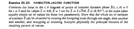
Homework Statement

MTW Ex 25.20 (see attachment MTW Ex25.20.png )

Relevant Equations

MTW Box 25.4 (27) See in attempt at solution

I am attempting to construct the locus in the r,θ diagram of points of constant dynamic phase S~(t,θ) for t=0 and for values ofL~=4M,E~=1


I begin with Equation (27) in Box 25.4 which is:



$\tilde S = - \tilde E t +\tilde L \theta$ $+ \int^r [\tilde E^2 - (1-\frac{2M}{r})(1+\frac{\tilde L^2}{r^2}]^\frac{1}{2}(1-\frac{2M}{r})^{-1}]dr$



Rewriting, using the chosen values $\tilde L=4M, \tilde E=1, t= 0$ :



$\tilde S = +\tilde 4M \theta$ $+ \int^r [1 - (1-\frac{2M}{r})(1+\frac{16M^2}{r^2}]^\frac{1}{2}(1-\frac{2M}{r})^{-1}]dr$



For points of constant dynamic phase $\tilde S = 0$, I get



$4M \theta = \int^r [1 - (1-\frac{2M}{r})(1+\frac{16M^2}{r^2}]^\frac{1}{2}(1-\frac{2M}{r})^{-1}dr$

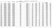
The integral looks pretty horrendous so I tried an alternative approach in which I plotted the curve on a spreadsheet and then used the spreadsheet to calculate the area under the curve for $\infty$ to$\frac{r}{2M}$ for a range of values from large $\frac {r}{2M}$ to $\frac {r}{2M} = 4$. I know that the values I produce are missing the constant value of the area under the curve from $\infty$ to$\frac{r}{2M}$ but I don't think that's a problem.

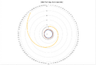
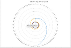
The result is attached (MTW Ex 25.20 Pt2.pdf)

So - Is this the correct curve?

I've tried tracing out this curve and rotating the tracing (about the Origin?) but I can't see how this produces a family of curves for $\tilde S$

Can anyone shed any light on this?


Regards


Terry W

 

[TSny]

$4M \theta = \int^r [1 - (1-\frac{2M}{r})(1+\frac{16M^2}{r^2}]^\frac{1}{2}(1-\frac{2M}{r})^{-1}dr$

The argument of the square root simplifies nicely. A computer algebra system will handle the integration.

 

[TerryW]

Hi TSny

Lovely to hear from you again. Hope you are keeping well.

I've used my spreadsheet to do the integration and then I hit on the idea of plotting my results on a radar chart where the result of the integration is the angle and the path is rendered by the value of r/2M plotted on the radial spines. I've done a rough plot so far and it has all the characteristics you'd expect - the path spirals in towards 4M. You can even see in the dataset that as you approach 4M the spiralling levels off (consistent with the plateauing of the potential at 4M.) I'm going to do a bit more work to make the plot more accurate (using more data points) and then I'll post it.

I wonder how early readers of MTW handled this problem. Back in the early 70's there were no spreadsheets and time on a computer was hard to come by. I note on page 677 Fig 25.6, is attributed to Prof R H Dicke who had produced the plot of a function using a digital calculator. Given that I bought my MTW in 1973, that must have been a pretty rudimentary machine!

Regards


TerryW

 

[TSny]

Hi TSny

Lovely to hear from you again. Hope you are keeping well.

Thanks, Terry. I'm doing well. It's nice to know you're still moving forward nicely with MTW.

I've used my spreadsheet to do the integration and then I hit on the idea of plotting my results on a radar chart where the result of the integration is the angle and the path is rendered by the value of r/2M plotted on the radial spines. I've done a rough plot so far and it has all the characteristics you'd expect - the path spirals in towards 4M. You can even see in the dataset that as you approach 4M the spiralling levels off (consistent with the plateauing of the potential at 4M.) I'm going to do a bit more work to make the plot more accurate (using more data points) and then I'll post it.

Sounds good. I've made some similar plots. I used the closed-form solutions for $\theta(r)$ obtained by letting Mathematica do the $r$-integration in equation (27) on page 649. Then I used Mathematica to do the plots. It will be interesting to see if we're getting similar results. Sounds like my plots are at least qualitatively in agreement with yours!

I wonder how early readers of MTW handled this problem. Back in the early 70's there were no spreadsheets and time on a computer was hard to come by. I note on page 677 Fig 25.6, is attributed to Prof R H Dicke who had produced the plot of a function using a digital calculator. Given that I bought my MTW in 1973, that must have been a pretty rudimentary machine!

I was wondering the same thing. (I purchased my MTW in '75. Pretty close!) Problem 25.20 must have been a tedious exercise back then. From the problem statement, I guess the authors expected you to plot one typical constant-$S$ curve by hand and then rotate this curve in equal increments to generate a family of constant-$S$ curves. Thanks for pointing out the reference to Dicke.

 

[TerryW]

My spreadsheet is now working well and I have plotted the orbit of a particle starting the integral at r/M = 193. I figured out a way to get Excel to produce a radial plot using some macros - I just haven't been able to get rid of the line joining the beginning of one of the orbit segments and the end.

I don't think the plot is quite right near to the centre when r/2M is approaching 4 but maybe this is a result of the 'integration' becoming a bit inaccurate when r/2M is rising rapidly. I can play with my model to see if what happens if I make the values for 'drain the 'integration' smaller in the region of r/2M = 4.

How does this compare with your results?

Regards


Terry

 

[TSny]

For the case $\tilde E = 1$ and $\tilde L = 4M$, I obtained the following $r$ - $\theta$ plots for the "surfaces" of constant dynamic phase $S$ (according to equation (27), box 25.4).

The axes are scaled to represent values of $r/M$. From this plot, you can get an idea of the shapes of particle trajectories corresponding to the given values of $\tilde E$ and $\tilde L$. The trajectories intersect the lines of constant $S$ at right angles. To test this, I numerically solved equation (25.41) to generate a particular trajectory and added it to the plot above:

The trajectory spirals asymptotically to $r = 4M$ [edited]. Your trajectory also spirals, but your trajectory is more circular for large values of r. My graphs above only go out to $r = 30 M$. Here's a graph that includes greater values of $r$.

Page 662 of MTW describes different trajectories for different values of $\tilde L$ and $\tilde E$. If I understand it, $\tilde E = 1$ corresponds to a particle falling in from $r = \infty$ with zero initial speed.

 

[TerryW]

Our different plots are not exactly alike - I'll have a think and get back to you. I'll see if I can do something to replicate your generation of the trajectory. I really like what you have done!

Terry

 

[TerryW]

I've had my think and run my model for a value of r/2M = 163 and found that my curve spirals 5+ times before it reaches r/2M = 4. I've attached a screenshot of my initial data. I assume that the result of the integral is an angle given in radians. I think that the spiralling arises because even at $r = \infty$ the particle has a velocity perpendicular to the radius, giving it the angular momentum $\tilde L$.

I'm going to produce an additional curve for a slightly increased value of $\tilde E$ to see if I can replicate the trick used on page 643 works and produces a trajectory.

To test this, I numerically solved equation (25.41) to generate a particular trajectory and added it to the plot above:

I'll also see if I can do this.

Cheers


Terry

 

[TSny]

I've had my think and run my model for a value of r/2M = 163 and found that my curve spirals 5+ times before it reaches r/2M = 4. I've attached a screenshot of my initial data.

The only thing I see that might be an error in your table is that the integrand should have an overall factor of 1/L = 1/4. This comes from solving equation (27), page 649, for $\theta$ when $t = 0$ and $S = 0$. This will slow down the rotation of your curve.

The case $L = 4$, $E = 1$ is special. The integral in (27) can be done in closed form to get $\theta = \sqrt{r/(2M)} + \tanh^{-1}(\sqrt{2M/r}) + {\rm const}$ . The constant doesn't matter, we can let it equal zero. Or, you could choose the constant so that this formula agrees with your data for $\varphi$ when $r/M = 4$.

I assume that the result of the integral is an angle given in radians. I think that the spiralling arises because even at $r = \infty$ the particle has a velocity perpendicular to the radius, giving it the angular momentum $\tilde L$.

Yes, I think that's right.

I'm going to produce an additional curve for a slightly increased value of $\tilde E$ to see if I can replicate the trick used on page 643 works and produces a trajectory.

That would be interesting.

 

[TerryW]

Hi TNsy

I'm still working on this, albeit slowly. (It's Spring so I need to get my vegetable seedlings going for one thing)

The case L=4, E=1 is special. The integral in (27) can be done in closed form to get θ=r/(2M)+tanh−1⁡(2M/r)+const

I have worked through (27) and derived the same answer as you (don't know why the square root signs have disappeared in the quote) but that immediately gave me a problem. I've added $\theta = \sqrt{r/(2M)} + \tanh^{-1}(\sqrt{2M/r}) + {\rm const}$ to my spreadsheet and found that the values of $\theta$ increase as $r/2M$ increases for the closed form integral whereas my computed integral decreases from r/2M = 4 to higher values (which you'd expect from the shape of the curve. I have noticed however that apart from the smallest values of r/2M, where my computed integral begins to get a bit inaccurate,the differences between the two values of $\theta$ are the same (save a multiple of -1) so it may be that they are the same curve or or a mirror image of each other.

That would be interesting.

I've had a go at this but so far, exploring only values of $\tilde E > 1$ the results haven't been encouraging. I'm going to try a few more values with $\tilde E < 1$ to see if anything begins to emerge. So I'm going to keep plugging away at this. I'll post again when I've done a bit more work.


Regards


TerryW

 

[TSny]

I have worked through (27) and derived the same answer as you (don't know why the square root signs have disappeared in the quote) but that immediately gave me a problem. I've added $\theta = \sqrt{r/(2M)} + \tanh^{-1}(\sqrt{2M/r}) + {\rm const}$ to my spreadsheet and found that the values of $\theta$ increase as $r/2M$ increases for the closed form integral whereas my computed integral decreases from r/2M = 4 to higher values (which you'd expect from the shape of the curve. I have noticed however that apart from the smallest values of r/2M, where my computed integral begins to get a bit inaccurate,the differences between the two values of $\theta$ are the same (save a multiple of -1) so it may be that they are the same curve or or a mirror image of each other

I believe you are getting the correct shape now. I took the first 11 points from your data table in post #8. I divided your angles by 4 to account for the missing overall factor of 1/L in the integrand in your table (mentioned in post #9). Here's what I get for a comparison between your data and the exact graph:

The brown curve is your data and the blue is $\theta = \sqrt{r/(2M)} + \tanh^{-1}(\sqrt{2M/r}) + {\rm const}$. I did flip your data over (mirror image) and rotated the graphs to have $\theta = 0$ at r/M = 4. They match well considering the step size of your numerical integration.

 

[TerryW]

Thanks for doing this. I'll carry on with my attempt to get the path by the 'interference' method.

 

[TerryW]

I've abandoned the attempt to get a path using the 'interference' method. There is a problem creating curves for values of $\tilde E < 0$ because the particle ends up at distances r/M >4, they don't have the energy to scale the full height of the potential, so the interesting part of the curve can't emerge. As an alternative, I adapted my spreadsheet to perform the integral of Eq 25.41 and have produced a curve similar to yours. See attachment. I'm currently exploring ways of actually performing the integration analytically (I now have φ as a function of u but I haven't yet worked out how to turn $\phi (u)$ into $\phi (r/M)$)

 

[TerryW]

Hi TSny

I think I've cracked it now. Equation 25.42, for the special values of $\tilde E= 1$, $L \dagger = 4$, has the 'analytic' solution:

$\phi = -4 \sqrt 8 ln(tan(\frac{1}{2}arcos(2 \sqrt(\frac{M}{r}))))$

I've used my spreadsheet to produce the orbits for the computed integral and the orbit for the 'analytic' integral. The two curves are very similar, though the computed solution has more rotations in the inner core. I reckon that this is down to the fact that my computed integral becomes less accurate, with slightly lower values for the integral, as the curve of the integrand gets steeper. At the higher values of r/M, the values for the integral are quite close.

I'm going to do a bit more work to explore the discrepancy between my calculated curve and the 'analytic' curve to see if I can find a satisfactory explanation.

Cheers

TerryW

 

[TSny]

I think I've cracked it now. Equation 25.42, for the special values of $\tilde E= 1$, $L \dagger = 4$, has the 'analytic' solution:

$\phi = -4 \sqrt 8 ln(tan(\frac{1}{2}arcos(2 \sqrt(\frac{M}{r}))))$

The result for $\phi$ from (25.42) can be expressed in different, but equivalent, ways. I found the following expressions: $$\phi = -\sqrt{8}\tanh^{-1}\left(2\sqrt{\frac{M}{r}}\right)$$ or $$\phi = \sqrt{2}\ln\left( \frac{1-2\sqrt{\frac{M}{r}}}{1+2\sqrt{\frac{M}{r}}}\right).$$These would agree with your expression if your expression didn't have the overall factor of 4. Since $L^{\dagger} = 4$, I wonder if one of us has dropped or added an extra factor of $L^{\dagger}$.

 

[TerryW]

I'm fairly confident about the factor 4 in my expression. The results from using this expression for $\phi$ with the factor 4 are very close to my original computed values. Without the factor 4, the discrepancy would be problematic.

I'll see if I can wrangle my expression for $\phi$ into yours.

 

[TSny]

Here's how I get my result. Equation (25.42) reads $$\left(\frac{du}{d \phi}\right)^2 = \frac{\tilde{E}^2 - (1-2u)(1+{{L^\dagger}}^2)}{{L^{\dagger}}^2},$$ where $u = M/r$. [Edit: The last factor in the numerator on the right should be $(1+{{L^\dagger }}^2u^2)$ instead of $(1+{{L^\dagger}}^2)$.]

Rearranging and letting $\tilde{E} = 1, L^\dagger = 4$, I get $$d\phi = \pm 2\sqrt{2} \frac{du}{\sqrt{u}(1-4u)}.$$ The $\pm$ just corresponds to clockwise or counterclockwise orbit.

Integrating, $$\phi = \pm \sqrt{2} \ln \left( \frac{1+ 2 \sqrt{u}}{1-2\sqrt{u}}\right) + \rm {const}.$$ This is equivalent to your result in post #14 except for a factor of 4. When taking the square root of both sides of (25.42), did you happen to forget to take the square root of ${L^{\dagger}}^2$ in the denominator of the right side of (25.42)?

 

[TerryW]

Hi TSny

I've checked my workings and have found the rogue factor of 4! I had also been doing some work to reconcile the differences between my computed integral and the analytic integral and was having a problem explaining why the analytic integral was greater than the computed integral. Removing the factor 4 fixed the problem!

Rearranging and letting E~=1,L†=4, I get dϕ=±22duu(1−4u).

I'm with you up to here but I then used a substitution, let $4u = Cos^2\theta$.
It was the factor 4 in $4du =-2Cos \theta Sin \theta$ that went adrift.

What happened to the factor $(\sqrt u)^{-1}$ in your integration? I think you will find that if you take the derivative wrtu of your solution, you won't get back to the original integrand.

Cheers


TerryW

 

[TSny]

Hi TSny

I've checked my workings and have found the rogue factor of 4! I had also been doing some work to reconcile the differences between my computed integral and the analytic integral and was having a problem explaining why the analytic integral was greater than the computed integral. Removing the factor 4 fixed the problem!

Great!

I'm with you up to here but I then used a substitution, let $4u = Cos^2\theta$.
It was the factor 4 in $4du =-2Cos \theta Sin \theta$ that went adrift.

Ok. I'm glad the pesky 4 has vanished.

What happened to the factor $(\sqrt u)^{-1}$ in your integration? I think you will find that if you take the derivative wrtu of your solution, you won't get back to the original integrand.

I get back the orginal integrand: $$\phi =\sqrt{2} \ln \left( \frac{1+ 2 \sqrt{u}}{1-2\sqrt{u}}\right) = \sqrt{2}\left[\ln(1+2\sqrt{u}) - \ln(1-2\sqrt{u}) \right]$$ So, $$\frac{d\phi}{du} = \sqrt{2}\left[ \frac{1}{1+2\sqrt{u}}\cdot \frac{1}{ \sqrt{u}} - \frac{1}{1-2\sqrt{u}}\cdot \left(-\frac{1}{ \sqrt{u}} \right) \right] = \frac{2\sqrt{2}}{\sqrt{u}(1-4u)}$$

 

[TerryW]

Sorry, that was a bit sloppy on my part!

I feel that there isn't much else to be extracted from this problem - but I have just one question I'm going to look at before I move on. That is: Why does $\frac {\partial{ \tilde S}}{\partial{ \tilde L}}$ produce 'the shape of the orbit' and why is this 'constructive interference'?
Let me have a think about this - I'll drop a new post if I can't figure it out.

Cheers


TerryW

 

[TerryW]

Hi TSny

I've now figured out the reasoning behind equations 28 & 29 in Box 25.4 - I just have one issue left which I haven't been able to resolve. It comes from the picture you posted in #6 of the orbit of the particle, which is a line that is normal to the wavefronts it crosses. I thought it ought to be possible to derive equation 28 from this diagram but haven't been able to show this. Have you considered this? I expect that if you have, you'll have found the answer!

Regards


TerryW

 

[TSny]

I thought it ought to be possible to derive equation 28 from this diagram but haven't been able to show this.

From Hamilton-Jacobi theory, the momentum $\boldsymbol p$ of the particle is equal to the gradient of the action $S$ $$\boldsymbol p = \boldsymbol{\nabla}S.$$ Thus, $\boldsymbol p$ is perpendicular to the surface of constant $S$ that passes through the location of the particle. Since $\boldsymbol p$ is tangent to the trajectory of the particle, the trajectory crosses the surfaces of constant $S$ at right angles to the surfaces.

So, a small displacement $\boldsymbol{dr}$ along the trajectory has the same direction as $\boldsymbol{\nabla}S$ $$ \boldsymbol{dr} \sim \boldsymbol{\nabla}S,$$ where $\sim$ means the two sides have the same direction. For motion in a plane using polar coordinates, we can write this as $$dr \, \hat r + r d\theta \,\hat \theta \sim \frac{\partial S}{\partial r} \hat r + \frac{\partial S}{r \partial \theta} \hat \theta.$$ In terms of ratios, this gives $$\left[ \frac {rd\theta}{dr}\right]_{\rm trajectory} = \frac{\partial S / r \partial \theta}{\partial S / \partial r}$$ or $$\left[ \frac {d\theta}{dr}\right]_{\rm trajectory} = \frac 1 {r^2} \frac{\partial S / \partial \theta}{\partial S / \partial r}$$ This is the equation that yields the trajectory. For example, in Box 21.4 equation (6) on page 646, we have $S$ for the Kepler problem: $$S = -Et +L\theta + \int^r \left[2 \left(E + \frac M r - \frac {L^2}{2r^2}\right)\right]^{1/2}dr.$$ Thus, we find the differential equation for the orbit: $$\left[ \frac {d\theta}{dr}\right]_{\rm trajectory} = \frac 1 {r^2} \frac{\partial S / \partial \theta}{\partial S / \partial r} = \frac {L}{r^2\left[2\left(E + \frac M r - \frac {L^2}{2r^2}\right)\right]^{1/2}}.$$ Separating variables and integrating yields the orbit given in equation (7), page 646.

Repeating for the Schwarzschild orbit, where $S$ is given in equation (27) page 649, you get the orbit equation (28).

 

[TerryW]

Hi Tony,

You really are a star!

Thanks.

TerryW