Numerical Solution to Schrodinger Equation w/ Coulomb Potential

[Tertius]

Homework Statement

I am trying to numerically solve the time-independent Schrödinger equation for the tunneling problem encountered in fusion processes (with a Coulomb barrier), specifically avoiding the use of the WKB approximation.

Relevant Equations

Schrodinger Equation
Coulomb Potential

I am doing this to have my own solution for customization and understanding. I also want to manually check the WKB approximation accuracy at various energies against this static solution.

I've split the problem into 3 regions and am solving it in 1D, but am having problems with how to define the initial boundary of Region 1.
$$r_{ctp}$$ is the classical turning point where incoming kinetic energy E equals coulomb potential V.
$$r_{nuc}$$ is the point where the nuclear strong force takes over at approximately the nuclear radius.

Region 1:
$$-\infty < x <= r_{ctp}$$
Region 1 has some of V(x) before reaching $r_{ctp}$.
Equation:
$$-\frac{\hbar^{2}}{2m} \frac{d^{2}}{dx^{2}} \psi_I(x) +V(x)\psi_I(x)=E\psi_I(x)$$
BCs:
$$\psi_I(-100) = 0$$
$$\psi_I'(-100) = 0.0001$$ (this is nonsense, and it propagates through the solutions).
If it is set to 0, then the solution is trivially 0. But the wave function should approach 0 going to $-\infty$.

Region 2:
$$r_{ctp} < x <= r_{nuc}$$
Region 2 has negative kinetic energy because E < V.
Equation:
$$-\frac{\hbar^{2}}{2m} \frac{d^{2}}{dx^{2}} \psi_{II}(x) +V(x)\psi_{II}(x)=E\psi_{II}(x)$$
BCs:
$$\psi_I(r_{ctp}) = \psi_{II}(r_{ctp})$$
$$\psi_I'(r_{ctp}) = \psi_{II}'(r_{ctp})$$

Region 3:
$$r_{nuc} < x <= 0$$
Region 3 is 'freely propagating' where $V(x)=0$
Equation:
$$-\frac{\hbar^{2}}{2m} \frac{d^{2}}{dx^{2}} \psi_{III}(x) =E\psi_{III}(x)$$
BCs:
$$\psi_{II}(r_{nuc}) = \psi_{III}(r_{nuc})$$

$$\psi_{II}'(r_{nuc}) = \psi_{III}'(r_{nuc})$$

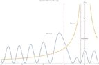
This setup is producing the attached graph using NDSolve in Mathematica.

The two questions i have are:
1) what are the appropriate BCs for Region 1?
2) why is the Region 2 solution oscillatory when it should be exponential? Usually that's a minus sign problem but wondering if there is something else going on.

Thanks

 

[Tertius]

I figured out where my approach was wrong. The boundary conditions for this are a little tricky because it is not a bound system.
So I discretized it manually and just solved $$H\psi = E\psi$$, where E is the kinetic energy of the incoming particle. E in this case is just a single eigenvalue because it is not a bound system, so it is possible to solve it as a simplified linear system as $$(H-EI)\psi = 0$$. This made it fast and give the same answer. But I did need to give the LinearSolver a small non-zero initial wave function value so it didn't give the trivial answer. Hope this helps someone.