KDPhysics
- 73
- 24
- TL;DR
- I have been trying to find a numerical solution to the Rayleigh Plesset equation (for a sonoluminescing bubble) using a Python code. Read up here if you need to refresh on this (surprisingly) unknown field: https://en.m.wikipedia.org/wiki/Sonoluminescence
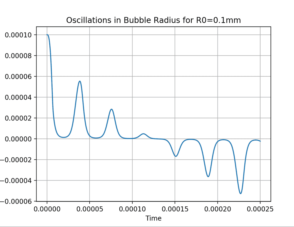
However, the python code seems to give a strange output. Please, gods of computational physics help me...
I have been trying to numerically solve the Rayleigh Plesset equation:
$R\ddot{R} + \frac{3}{2}(\dot{R})^2=\frac{p_g-p_0-p(t)}{\rho_l}-4\mu\frac{\dot{R}}{R}-\frac{2\gamma}{\rho_lR}$
using the odeint python function. The code is given below:
Wh
 en i run the code, I get a very strange output.
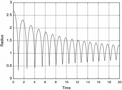
It should look more like this:

[1]: https://i.stack.imgur.com/aTc3j.png
[2]: https://i.stack.imgur.com/fQ9J8.gif
EDIT:
Ok, I've been working on the code for a while, and I think I have found the mistake. I was using an approximate form of the equation. For anyone interested in the correct code, here it is (feel free to edit it if you want, I am bad at writing efficient code XD).
I rescaled the axes so that the marks wouldn't overlap, and the results should coincide with past literature.
$R\ddot{R} + \frac{3}{2}(\dot{R})^2=\frac{p_g-p_0-p(t)}{\rho_l}-4\mu\frac{\dot{R}}{R}-\frac{2\gamma}{\rho_lR}$
using the odeint python function. The code is given below:
Python:
import numpy as np
from matplotlib import pyplot as plt
from scipy.integrate import odeint

# define equations
def equation(y0, t):
    R, u = y0
    return u, (P_g-P_0-1317000*np.sin(2*np.pi*26500*t)-2*sigma/R)/(R*rho)-4*miu*u/(R**2)-3*u**2/(2*R)

def plot_results(time, R):
    plt.plot(time, R)

    s = " for R0=" + str(R_0*1000) + "mm"
    plt.title("Oscillations in Bubble Radius" + s)
    plt.xlabel("Time")
    plt.ylabel("Radius of bubble")
    plt.grid(True)
    plt.show()

# parameters
time = np.arange(0, 0.0005, 0.000000025)
rho = 1000
sigma = 0.0725
miu = 8.9*10**(-4)
P_g = 2330
P_0 = 10000

# initial conditions
R_0 = 0.0001
u_0 = 0

R_1 = odeint(equation, [R_0, u_0], time)

R = R_1[:,0]

plot_results(time, R)
Wh
It should look more like this:
[1]: https://i.stack.imgur.com/aTc3j.png
[2]: https://i.stack.imgur.com/fQ9J8.gif
EDIT:
Ok, I've been working on the code for a while, and I think I have found the mistake. I was using an approximate form of the equation. For anyone interested in the correct code, here it is (feel free to edit it if you want, I am bad at writing efficient code XD).
Python:
import numpy as np
from matplotlib import pyplot as plt
from scipy.integrate import odeint

# define equations
def equation(y0, t):
    R, u = y0
    return u, (P_g-P_0-1317000*np.cos(2*np.pi*26500*t)-2*sigma/R-4*miu*u/R+(2*sigma/R_0+P_0-P_g)*(R_0/R)**(3*k))/(R*rho)-3*u**2/(2*R)

#define plot
def plot_results(mtimes, R):
    plt.plot(mtimes, R)

    s = " for R0=" + str(R_0*10**6) + "$\mu$m"
    plt.title("Oscillations in Bubble Radius" + s)
    plt.xlabel("T/$\mu$s")
    plt.ylabel("R/$\mu$m")
    plt.grid(True)
    plt.show()

# parameters
time = np.arange(0, 0.00002, 0.00000000025)
rho = 1000
sigma = 0.0725
miu = 8.9*10**(-4)
P_g = 2330
P_0 = 10000
k = 1.33

# initial conditions
R_0 = 0.0000026
u_0 = 0

R_1 = odeint(equation, [R_0, u_0], time)

R = R_1[:,0]*10**6
mtimes = time*10**6

#plot the results
plot_results(mtimes, R)
I rescaled the axes so that the marks wouldn't overlap, and the results should coincide with past literature.
Attachments
Last edited:
