- 2,186
- 2,694
I want to solve the heat equation numerically. The equation is: $$k \dfrac{\partial^2 T}{\partial x^2} = \dfrac{\partial T}{\partial t}.$$ This is a parabolic PDE.
Following this pdf (specifically, equation 7 given on page 3), I wrote the following Python function to implement the explicit algorithm:
Our college Professor gave us a sample problem to test our programs. The given values are as follows:
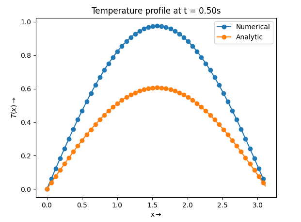
And I get this graph:

Obviously, the numerical solution doesn't match the analytic solution.
I double-checked my function, and there seems to be no error. But there is an error somewhere, right?
If I print
Ignore the
Any idea where the problem is occurring?
Following this pdf (specifically, equation 7 given on page 3), I wrote the following Python function to implement the explicit algorithm:
Python:
import numpy as np

def heat_equation_explicit(t0, t_end, dt, dx, k, initial_profile):
    """
    Solves the heat equation using explicit algorithm.

    Parameters
    ----------
    t0 : float
        The start of time.
    t_end : float
        The end of time.
    dt : float
        Time step.
    dx : float
        Step size on x-axis.
    k : float
        Diffusivity.
    initial_profile : numpy.ndarray
        The initial heat profile for all values of x over which the solution has to be calculated,
        (i.e. T(x, 0) ∀ x ∈ np.arange(x0, x_end, dx)). The first and the  last elements should be the
        boundary values, i.e. T(x0, t) and T(x_end, t), which will remain constant with time.

    Returns
    -------
    numpy.ndarray
        The heat profile at t = t_end.

    """

    # Number of steps:
    num_t = round((t_end - t0) / dt)
    num_x = np.size(initial_profile)

    old_profile = initial_profile

    global finalProfile_numerical

    lamb = (k * dt) / (dx ** 2)

    for j in range(0, num_t):

        # Initialise the variable:
        finalProfile_numerical = np.zeros(num_x)

        # Keep the boundary values at the two ends:
        finalProfile_numerical[0] = initial_profile[0]
        finalProfile_numerical[-1] = initial_profile[-1]

        # Compute the new profile:
        for i in range(1, num_x - 1):

            u_old_iPlus1 = old_profile[i + 1]
            u_old_iMinus1 = old_profile[i - 1]

            finalProfile_numerical[i] = old_profile[i] + lamb * (u_old_iPlus1 - 2 * old_profile[i] + u_old_iMinus1)

        old_profile = finalProfile_numerical

return finalProfile_numerical- ##x \in [0, \pi]##
- ##T(0, t) = T(\pi,t) = 0##
- ##T(x,0) = \sin x##
- ##k = 0.05##
- Analytical solution: ##T(x,t) = \exp(-t) \sin x##
- I have to compute the final profile at ##t = 0.5s.##
Python:
import math
import numpy as np
import matplotlib.pyplot as plt

x0 = 0
xEnd = math.pi
dx = math.pi / 100

t0 = 0
tEnd = 0.5
dt = 0.01

k = 0.05

xVal = np.arange(x0, xEnd, dx)

# Values of T(x, 0) at all x. Includes T(x0, t) at the beginning, and T(x_end, t) at the end.
initialProfile = np.sin(xVal)

finalProfile_numerical = heat_equation_explicit(t0, tEnd, dt, dx, k, initialProfile)
finalProfile_analytic = math.exp(-0.5) * np.sin(xVal)

# Plot the numerical solution:
plt.plot(xVal, finalProfile_numerical, '-o', label="Numerical", markevery=2)

# Plot the analytical solution:
plt.plot(xVal, finalProfile_analytic, '-o', label='Analytic', markevery=2)

plt.xlabel(r'x$\rightarrow$')
plt.ylabel(r'$T(x)\rightarrow$')
plt.title("Temperature profile at t = " + f'{tEnd:.2f}' + "s")
plt.legend(loc='best')
plt.show()Obviously, the numerical solution doesn't match the analytic solution.
I double-checked my function, and there seems to be no error. But there is an error somewhere, right?
If I print
final_profile_numerical / final_profile_analytic, I get:
Code:
[       nan 1.60800745 1.60800745 1.60800745 1.60800745 1.60800745
 1.60800745 1.60800745 1.60800745 1.60800745 1.60800745 1.60800745
 1.60800745 1.60800745 1.60800745 1.60800745 1.60800745 1.60800745
 1.60800745 1.60800745 1.60800745 1.60800745 1.60800745 1.60800745
 1.60800745 1.60800745 1.60800745 1.60800745 1.60800745 1.60800745
 1.60800745 1.60800745 1.60800745 1.60800745 1.60800745 1.60800745
 1.60800745 1.60800745 1.60800745 1.60800745 1.60800745 1.60800745
 1.60800745 1.60800745 1.60800745 1.60800745 1.60800745 1.60800745
 1.60800745 1.60800745 1.60800745 1.60800745 1.60800745 1.60800745
 1.60800745 1.60800745 1.60800745 1.60800745 1.60800745 1.60800745
 1.60800745 1.60800745 1.60800745 1.60800745 1.60800745 1.60800745
 1.60800745 1.60800745 1.60800745 1.60800745 1.60800746 1.60800746
 1.60800747 1.60800748 1.60800752 1.60800757 1.60800769 1.60800788
 1.60800825 1.60800886 1.60800999 1.60801179 1.60801496 1.60801993
 1.6080283  1.60804126 1.60806232 1.60809452 1.60814542 1.60822265
 1.60834263 1.60852485 1.60880718 1.60924297 1.60993333 1.61105178
1.61296191 1.61650076 1.6242027 1.64872127]nan in the front. Interestingly, note that ##1 / \exp(-0.5) = 1.648##.Any idea where the problem is occurring?