Discussion Overview
This thread discusses various unsolved statistics questions from other sites, focusing on the interpretation and implications of statistical concepts, particularly regarding distributions and probabilities. The scope includes theoretical questions and mathematical reasoning.
Discussion Character
- Exploratory
- Technical explanation
- Debate/contested
- Mathematical reasoning
Main Points Raised
- One participant questions whether the variable x1-x2 can be concluded to be normally distributed based solely on provided means and standard deviations, suggesting that additional information about the populations is necessary.
- Another participant argues that if means and standard deviations are given, it is often implied that the random variables are normally distributed, but cautions against making such assumptions without explicit clarification.
- A different participant provides a mathematical derivation using Fourier Transform to show that the sum of two normal random variables is also normal, applying it to the specific means and standard deviations given in the original question.
- There is a suggestion that the original question may have been poorly formulated, leading to misunderstandings about the assumptions necessary for a correct answer.
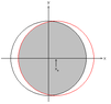
- In a separate question about the probability of the center of a circle being inside a triangle formed by three randomly chosen points on its circumference, one participant proposes a method involving geometric considerations and Monte Carlo simulations to arrive at a probability of 1/4.
- Another participant offers a different approach to the same problem, simplifying the situation by normalizing angles and using geometric reasoning to arrive at the same probability result.
- A new question is introduced regarding a sequence of independent binary random variables and the demonstration that their sum is uniformly distributed between 0 and 1, with one participant suggesting a Fourier Transform approach to the proof.
Areas of Agreement / Disagreement
Participants express differing views on the assumptions necessary for concluding normality in the first question, indicating a lack of consensus. The discussions on the probability problem show some agreement on the result, but the methods proposed vary. The question about the uniform distribution also remains open for discussion without a clear resolution.
Contextual Notes
Some discussions highlight the importance of clearly stating assumptions and the potential pitfalls of ambiguous questions. The mathematical steps in some arguments are not fully resolved, leaving room for further exploration.