Graph of time vs distance for sizing a motor for linear motion

[Travis T]

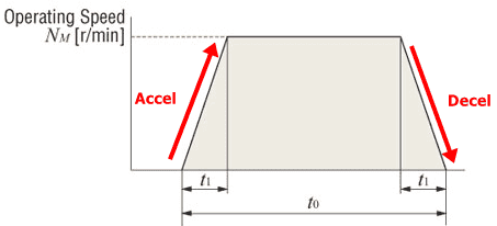
Hi, I'm sizing motor for a linear motion,
usually for the time distance graph would be looks like this,

however, how does the graph look like if the stroke is very short?
Example: velocity is 0.1m/s, acceleration is 1m/s2, moving stroke is 0.5mm, a cycle is within 0.05s
the application is to compensate positioning errors which is very small.

 

[Baluncore]

... the application is to compensate positioning errors which is very small.

The motor is inside a feedback loop, so the inertia of the motor, and the characteristics of the feedback loop will be very important to the performance.

... however, how does the graph look like if the stroke is very short?

You might consider using a piezo transducer to make the fine position correction.

 

[jrmichler]

I like to solve servo motion problems by making a simple hand sketch showing acceleration, velocity, and position. You want to move 0.5 mm in 0.05 seconds as precisely as practical. Start the calculations by assuming a constant acceleration move, as shown in the simple sketch below:

Since $Distance = 0.5 * a * t^2$, and we know both the distance and the time, we can solve for the acceleration and add that number to the sketch. This is a minimum acceleration move, which is a good place to start when you want precision or a fast move. The peak velocity is then $0.8 m/s^2 * 0.025 s = 0.02 m/s$. If the acceleration and peak velocity are within the servo specifications, then program that move, and check the response. Does it do what you want?

If it stops within your position tolerance, you are finished. If it oscillates to a stop, the next step is a finite jerk move. If that happens, post again and we can help you solve that problem.

 

[Travis T]

I like to solve servo motion problems by making a simple hand sketch showing acceleration, velocity, and position. You want to move 0.5 mm in 0.05 seconds as precisely as practical. Start the calculations by assuming a constant acceleration move, as shown in the simple sketch below:
View attachment 339044
Since $Distance = 0.5 * a * t^2$, and we know both the distance and the time, we can solve for the acceleration and add that number to the sketch. This is a minimum acceleration move, which is a good place to start when you want precision or a fast move. The peak velocity is then $0.8 m/s^2 * 0.025 s = 0.02 m/s$. If the acceleration and peak velocity are within the servo specifications, then program that move, and check the response. Does it do what you want?

If it stops within your position tolerance, you are finished. If it oscillates to a stop, the next step is a finite jerk move. If that happens, post again and we can help you solve that problem.

Is it Distance = 0.25 * a * t^2? instead of 0.5?
how do we get 0.8m/s^2?

 

[jrmichler]

Velocity is the integral of acceleration, or the area under the acceleration curve.
Similarly, position is the integral of velocity, or the area under the velocity curve.

Since the acceleration curve has a discontinuity, the integration is in two parts. The first part is from 0 to 0.025 seconds, the second part from 0.025 seconds to 0.05 seconds. The two parts are then summed to get the final velocity, which is zero. The curves help show that the acceleration is positive for halfway, and negative for the last halfway. The integral of the acceleration is the velocity, which increases to a maximum at the halfway point, then decreases to zero at the end.

It is important understand these concepts when doing motion control, and the diagrams help to understand the concepts. The diagrams are not very important for simple problems like this. They become much more important if you need, for example, a finite jerk motion profile to reduce position errors. The diagrams are also useful in a large engineering department to communicate to other engineers.

We get $0.8 m/s^2$ by solving $Distance = 0.5at^2$ as follows:
Distance = 0.25 mm (halfway to 0.5 mm) (distance from beginning to first discontinuity)
t = 0.025 second (halfway to 0.05 second) (time from beginning to first discontinuity)
The only unknown is the acceleration, so solve the equation for the acceleration.

 

[Travis T]

Velocity is the integral of acceleration, or the area under the acceleration curve.
Similarly, position is the integral of velocity, or the area under the velocity curve.

Since the acceleration curve has a discontinuity, the integration is in two parts. The first part is from 0 to 0.025 seconds, the second part from 0.025 seconds to 0.05 seconds. The two parts are then summed to get the final velocity, which is zero. The curves help show that the acceleration is positive for halfway, and negative for the last halfway. The integral of the acceleration is the velocity, which increases to a maximum at the halfway point, then decreases to zero at the end.

It is important understand these concepts when doing motion control, and the diagrams help to understand the concepts. The diagrams are not very important for simple problems like this. They become much more important if you need, for example, a finite jerk motion profile to reduce position errors. The diagrams are also useful in a large engineering department to communicate to other engineers.

We get $0.8 m/s^2$ by solving $Distance = 0.5at^2$ as follows:
Distance = 0.25 mm (halfway to 0.5 mm) (distance from beginning to first discontinuity)
t = 0.025 second (halfway to 0.05 second) (time from beginning to first discontinuity)
The only unknown is the acceleration, so solve the equation for the acceleration.

Thanks for the clear explanation.