How can I fix the dimensions mismatch in my split-step Fourier method code?

In summary: Plot input pulsefigure(1)plot(abs(u),'b');title('Input Pulse');xlabel('Time');ylabel('Amplitude');axis([-gridscale gridscale 0 tmax 0 zmax]), grid on%Solve nonlinear part (D=0)u = u.*exp(i*h*gamma*abs(u).^2);%Solve linear part in Fourier space (N=0)v = fft(u);D = i*s*omega.^2;v = v.*exp(h.*D);u = ifft(v);u =
  • #1
roam
1,271
12
I am trying to write a very basic Matlab code to preform the split-step Fourier method on the nonlinear Schrodinger equation:

$$\frac{\partial A(z,T)}{\partial z} = -i \frac{\beta_2}{2} \frac{\partial^2A}{\partial T^2} + i \gamma |A|^2 A \ \ (1)$$

I want the program to make 3D plots of Gaussian input pulses (##A(0, T) = \sqrt{P_0} exp (-T^2/(2T_0^2))##) propagating over different distances. It should look something like this:
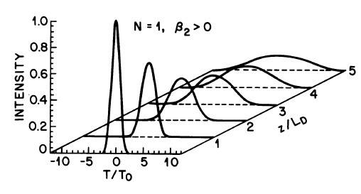
IjJ1x.jpg


Attempt:

Here is my code (I chose some dummy values to check whether the code is working):

Code:
    b=20; % in ps^2/km
    s=b/2; % dispersive term
    gamma = 2^(-10); % nonlinear term
   
    h=1000; % propagation stepsize
    N=100; % number of steps (Length traveled = h*N)
    dt=2^(-10); % time step
    P0=.00064; % input powr in watts
    A0=sqrt(P0); % Amplitude
    tau =- 4096e-12:1e-12: 4095e-12;
    t0=125e-12; % input pulse width in seconds
    omega=0.1:0.1:1.5;
   
    u=A0*exp((-tau.^2)/(2*t0).^2);  % Gaussian input pulse
   
    %Plot input pulse
    figure(1)
    plot(abs(u),'b');
    title('Input Pulse'); xlabel('Time'); ylabel('Amplitude');
   
   
    for n = 1:N
   
    %Solve nonlinear part (D=0)
    u = u.*exp(i*h*gamma*abs(u).^2);
    %Solve linear part in Fourier space (N=0)
    v = fft(u);
    D = i*s*omega.^2;
    v = v.*exp(h.*D); % analytical soln
    u = ifft(v); % back to real space
    u = u.*exp(i*gamma*abs(u).^2*h);
   
    end
   
    %Plot results
    figure(2);
    w=waterfall(x,t,u')
    set(w,'edgecolor','b');
    title('Evolution of pulse shapes');
    ylabel('distance (km)'), xlabel('Time (ps)'),zlabel('amplitude'); axis([-gridscale gridscale 0 tmax 0 zmax]), grid on

But the code doesn't work. There is no graph generated and I get the message that "Matrix dimensions must agree" I think because omega is a 1 by 15 row vector, and so is exp(v.*D), but v is a different size. How can I fix this?

Is the overall structure of the code correct or do we need to do this differently?

Any help would be greatly appreciated.

P.S.
The split-step Fourier method I am asked to use works by writing (1) as:

$$\frac{\partial A}{\partial z} = \left( \hat{D} + \hat{N} \right) A$$

With ##\hat{D} = -i (\beta_2 / 2) \partial^2 /\partial T^2## is the linear disperiosn operator while ##\hat{N} = i \gamma |A|^2## is the nonlinear operator. So for a step size ##h##, ##z \to z+h## we have

$$A(z,T) \to e^{h \hat{N}} A(z,t) \approx exp \Big[ ih \gamma |A(z,T)|^2 \Big] A(z,T).$$

$$\frac{\partial A(z,T)}{\partial z} = \hat{D} A(z,T)$$

becomes after temporal Fourier transform

$$\frac{\partial \tilde(A) (z, \Omega)}{\partial z} = \hat{D} (-i \Omega) \tilde{A} (z, \Omega)$$

an exact solution of which is ##e^{h \hat{D} (-i \Omega)} \tilde{A} (z, \Omega).##

Combining the two equations we get the following for a full integration step:

$$ \therefore \ A(z+h, T) = e^{h \hat{D}} e^{h \hat{N}} A(z,T) \approx FT^{-1} \Big[ e^{ih\beta_2 \Omega^2/2} FT [e^{ih \gamma |A(z,T)|^2} A(z,T)] \Big].$$
 
Physics news on Phys.org
  • #2
The frequencies appearing in D are governed by the FFT and depend on the size and length of the spatial grid. You have calculate them correctly, and take into account the special order of the FFT data in reciprocal space (momentum space in your case). See for instance chapter 12 of Numerical Recipes http://www.nrbook.com/a/bookcpdf.php

Also, I strongly advise against using the asymmetric split you are using. You should use ##e^{h \hat{D}/2} e^{h \hat{N}} e^{h \hat{D}/2}## or ##e^{h \hat{N}/2} e^{h \hat{D}} e^{h \hat{N}/2}##. Have a look at http://iopscience.iop.org/article/10.1088/0305-4470/39/12/L02
 
  • #3
DrClaude said:
The frequencies appearing in D are governed by the FFT and depend on the size and length of the spatial grid. You have calculate them correctly, and take into account the special order of the FFT data in reciprocal space (momentum space in your case). See for instance chapter 12 of Numerical Recipes http://www.nrbook.com/a/bookcpdf.php

Ok, so I realized that if the time step size is ##\Delta t##, the span time would be ##N.\Delta t##, so then the frequency step would be ##1/\Delta t## (this is ##\Omega## in my code), and the span would be ##1/N \Delta t##. Using this information I modified the code:

Code:
b = 20; % in ps^2/km
s = b/2; % dispersive term
gamma = 2^(-10); % nonlinear term

h = 0.5; % propagation stepsize
N = 100; % number of steps (L = h*N)
dt = 2^(-6); % time step as a power of 2
P0 = 89.7e-3; % input power in watts
A0  =sqrt(P0); % amplitude
tau = -N*dt : dt : N*dt;
t0 = 0.325; % input pulse width in picoseconds
omega = -1/(N*dt) : 1/dt : 1/(N*dt);
L = 1 % length of the fiber in km
d = linspace(0,L,L/h) % distance in km

ld = (t0/abs(b)).^2; % disperison length
ln = 1/(gamma*P0); % nonlinear length

u = A0*exp((-tau.^2)/((2*t0).^2));  % Gaussian input pulse

%Plot input pulse
figure(1)
plot(abs(u),'b');
title('Input Pulse'); xlabel('Time'); ylabel('Amplitude');

for n = 1:N

%Solve nonlinear part (D=0)
u = u.*exp(i*h*gamma*abs(u).^2);
%Solve linear part in Fourier space (N=0)
v = fft(u);
D = i*s*omega.^2;
v = v.*exp(h.*D); % analytical soln
u = ifft(v); % back to real space
u = u.*exp(i*gamma*abs(u).^2*h);

udata = [udata abs(u)]; tdata = [tdata tau];

end

%Plot results
figure(2);
w = waterfall(d,tdata,udata')
set(w,'edgecolor','b');

But I still get no graph, and I get the following error:

Code:
Error using horzcat
CAT arguments dimensions are not consistent.

Error in waterfall (line 57)
z = [z0*ones(size(x,1),1) z(:,1) z z(:,size(z,2))
z0*ones(size(x,1),2) ];

What is wrong here? :confused:

Also, in my code how do I exactly deal with the special order of the FFT data in reciprocal space? Do I need to be using the FFTSHIFT(...) syntax somewhere?
 
Last edited:
  • #4
Sorry, I meant to say that the span of time window is ##N \Delta T## so the frequency spacing is ##1/N \Delta T## and frequency span would be ##1/\Delta T##.

This is my new code:

Code:
h = 0.5*ld; % propagation step size
N = 100; % number of steps
dt = 2^(-6); % sample spacing as a power of 2

b = 20; % in ps^2/km
s = b/2; % dispersive term
gamma = 2^(-10); % nonlinear term
P0 = 89.7e-3; % input power in watts
A0  = sqrt(P0); % amplitude
t0 = 0.325; % input pulse width in picoseconds
tau = -N*dt : dt : N*dt;
omega = -1/(dt) : 1/(N*dt) : 1/(dt);

L = 1; % length of the fiber in km
d = linspace(0,L,L/h); % distance in km

ld = (t0/abs(b)).^2; % disperison length
ln = 1/(gamma*P0); % nonlinear length

u = A0*exp((-tau.^2)/((2*t0).^2));  % Gaussian input pulse

% Solve PDE:
udata = abs(u);
tdata = 0;for n = 1:N

%Solve nonlinear part (D=0)
u = u.*exp(i*h*gamma*abs(u).^2);
%Solve linear part in Fourier space (N=0)
v = fft(u);
v = fftshift(v);
D = i*s*omega.^2;
v = v.*exp(h.*D); % analytical solution in Fourier space
u = ifft(fftshift(v)); % back to real space
u = u.*exp(i*gamma*abs(u).^2*h);udata = [udata abs(u)];
udata = [];
tdata = [tdata tau];

end

% Plot results
figure(2);
w = waterfall(d,tdata,udata)
set(w,'edgecolor','b');
title('Evolution of pulse shapes');
ylabel('distance (km)'), xlabel('Time (ps)'),zlabel('amplitude'); axis([-gridscale gridscale 0 tmax 0 zmax]), grid on

I get the message that there is an error in "w = waterfall(d,tdata,udata)" and "dimensions do not agree" or "Index exceeds matrix dimensions" (but I checked the dimensions!).

So I tried the mesh syntax instead of waterfall, but I am getting a blank 3D plot. Why is that?
 
Last edited:
  • #5
roam said:
Sorry, I meant to say that the span of time window is ##N \Delta T## so the frequency spacing is ##1/N \Delta T## and frequency span would be ##1/\Delta T##.

This is my new code:

Code:
h = 0.5*ld; % propagation step size
N = 100; % number of steps
dt = 2^(-6); % sample spacing as a power of 2

b = 20; % in ps^2/km
s = b/2; % dispersive term
gamma = 2^(-10); % nonlinear term
P0 = 89.7e-3; % input power in watts
A0  = sqrt(P0); % amplitude
t0 = 0.325; % input pulse width in picoseconds
tau = -N*dt : dt : N*dt;
omega = -1/(dt) : 1/(N*dt) : 1/(dt);

L = 1; % length of the fiber in km
d = linspace(0,L,L/h); % distance in km

ld = (t0/abs(b)).^2; % disperison length
ln = 1/(gamma*P0); % nonlinear length

u = A0*exp((-tau.^2)/((2*t0).^2));  % Gaussian input pulse

% Solve PDE:
udata = abs(u);
tdata = 0;for n = 1:N

%Solve nonlinear part (D=0)
u = u.*exp(i*h*gamma*abs(u).^2);
%Solve linear part in Fourier space (N=0)
v = fft(u);
v = fftshift(v);
D = i*s*omega.^2;
v = v.*exp(h.*D); % analytical solution in Fourier space
u = ifft(fftshift(v)); % back to real space
u = u.*exp(i*gamma*abs(u).^2*h);udata = [udata abs(u)];
udata = [];
tdata = [tdata tau];

end

% Plot results
figure(2);
w = waterfall(d,tdata,udata)
set(w,'edgecolor','b');
title('Evolution of pulse shapes');
ylabel('distance (km)'), xlabel('Time (ps)'),zlabel('amplitude'); axis([-gridscale gridscale 0 tmax 0 zmax]), grid on

I get the message that there is an error in "w = waterfall(d,tdata,udata)" and "dimensions do not agree" or "Index exceeds matrix dimensions" (but I checked the dimensions!).

So I tried the mesh syntax instead of waterfall, but I am getting a blank 3D plot. Why is that?

Hii Bro..

Did you get a solution for this problem.

I am trying to solve a similar problem using ode45 in matlab..can you help me out.

Pavan
 
  • #6
roam said:
I get the message that there is an error in "w = waterfall(d,tdata,udata)" and "dimensions do not agree" or "Index exceeds matrix dimensions" (but I checked the dimensions!).
tdata and udata do not have the same size.
 

1. What is the Split-step Fourier method?

The Split-step Fourier method is a numerical technique used to solve partial differential equations (PDEs), particularly those that are non-linear and involve the propagation of waves. It involves breaking down the PDE into smaller steps that can be solved using the Fast Fourier Transform algorithm.

2. How does the Split-step Fourier method work?

The method involves splitting the PDE into two parts - a linear and a non-linear part. The linear part can be solved analytically while the non-linear part is solved using the Fast Fourier Transform algorithm. The solutions from both parts are then combined to give an approximate solution to the original PDE.

3. What are the advantages of using the Split-step Fourier method?

One of the main advantages of this method is its efficiency. By breaking down the PDE into smaller steps, it reduces the computational complexity and time required to solve the problem. It also has a high accuracy and can handle a wide range of PDEs, making it a versatile tool for scientists and engineers.

4. What are the limitations of the Split-step Fourier method?

While the method is efficient and accurate, it is not suitable for all types of PDEs. It works best for PDEs that are non-linear and involve wave propagation. It also requires the use of the Fast Fourier Transform algorithm, which may not be familiar to all scientists and engineers.

5. In what fields is the Split-step Fourier method commonly used?

This method is commonly used in fields such as optics, acoustics, and quantum mechanics, where PDEs involving wave propagation are prevalent. It is also used in signal processing and image processing, as well as in the simulation of physical systems in engineering and physics.

Similar threads

Replies
4
Views
304
  • Calculus and Beyond Homework Help
Replies
3
Views
768
  • MATLAB, Maple, Mathematica, LaTeX
Replies
1
Views
2K
  • MATLAB, Maple, Mathematica, LaTeX
Replies
5
Views
2K
  • Advanced Physics Homework Help
Replies
6
Views
1K
  • MATLAB, Maple, Mathematica, LaTeX
2
Replies
41
Views
8K
  • MATLAB, Maple, Mathematica, LaTeX
Replies
7
Views
2K
Replies
6
Views
1K
  • Calculus and Beyond Homework Help
Replies
2
Views
1K
  • MATLAB, Maple, Mathematica, LaTeX
Replies
3
Views
2K
Back
Top