Numerical methods for PV modeling

[nughii]

Homework Statement

How to solve the equation below using numerical methods

Relevant Equations

$$I=I_{pv}-I_o \left [ exp \Big( \frac{V+R_s I}{V_t a} \Big) - 1 \right ] - \frac{V+R_s I}{Rp}$$

Input parameter
$$I_{pv}= 8.2 A$$
$$I_{o=}9.8 e -8 A$$
$$R_s=0.221 \Omega$$
$$R_p=415.405 \Omega$$
$$a=1.3$$
$$V_t=21177.82 V$$

source (Villalva, Marcelo G. 2009. Comprehensive Approach to Modeling and Simulation of Photovoltaic Arrays. IEEE Transaction On Power Electronics, Vol. 24, No. 5)

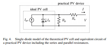
Fig 4 is the model of PV device. This is modeled by the I-V equation above.
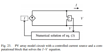
Fig 23 is the circuit model composed of only one current source. The value of the current is obtained by numerically solving the I–V equation. For every value of V , a corresponding I that satisfies the I–V equation is obtained.Is it possible to solve the equation using Runge Kutta method? Could you teach me how to do the first iteration using this method? Or, what numerical method should be used? Thank you...

 

[BvU]

Hello nughii, !

Is it possible to solve the equation using Runge Kutta method?

Runge-Kutta methods are used for differential equations. Your equation is an algebraic equation, for which one can use a numerical equation solver if an analytic solution is too cumbersome.

But first have a problem to solve: your I and your V are unknowns. So either you calculate an I-V curve $I=f(V)$ or you find a second equation.

For an I-V curve, a simple start is sucessive substitution: assume a value for I and use your equation as-is to calculate a (hopefully) better one.
(with V = 10 I get a sequence 8.168, 8.164, 8.1636
not sure what you mean with $I_0 =9.8 e -8$ A -- as you write it, it is 18.64 A but probably you mean $9.8 \times 10^{-8}$ A, in which case the sequence is 1, 8.175, 8.172
and: is Vt really so big: 21177.82 V ? )https://www.google.com/search?q=equ...4.69i57j0l7.9531j0j7&sourceid=chrome&ie=UTF-8https://www.google.com/search?rlz=1...13j0i8i7i30j0i8i7i10i30j0i13i5i30.3gQ-TVFbW1g

 

[Chestermiller]

It seems to me the bracketed term is going to be negligible, which leaves a linear relation between V and I.

 

[BvU]

Tried a few numerical values and realized what @Chestermiller saw straightaway: if the givens are correct, a linear (or a Taylor series) approximation is just fine.

 

[nughii]

Hello nughii, !

Runge-Kutta methods are used for differential equations. Your equation is an algebraic equation, for which one can use a numerical equation solver if an analytic solution is too cumbersome.

But first have a problem to solve: your I and your V are unknowns. So either you calculate an I-V curve $I=f(V)$ or you find a second equation.

For an I-V curve, a simple start is sucessive substitution: assume a value for I and use your equation as-is to calculate a (hopefully) better one.
(with V = 10 I get a sequence 8.168, 8.164, 8.1636
not sure what you mean with $I_0 =9.8 e -8$ A -- as you write it, it is 18.64 A but probably you mean $9.8 \times 10^{-8}$ A, in which case the sequence is 1, 8.175, 8.172
and: is Vt really so big: 21177.82 V ? )https://www.google.com/search?q=equ...4.69i57j0l7.9531j0j7&sourceid=chrome&ie=UTF-8https://www.google.com/search?rlz=1...13j0i8i7i30j0i8i7i10i30j0i13i5i30.3gQ-TVFbW1g

Thank you for the explanation...

1. Yes, I mean the value of $I_0$ is $9.8 \times 10^{-8}$ A.
2. I am sorry, the value of $Vt$ is $1.38 V$.
3. I think, if I'm not mistaken, I can use the second equation if the PV is coupled with a resistor. So, the second equation is $V=I * R$.

For an I-V curve, a simple start is sucessive substitution: assume a value for I and use your equation as-is to calculate a (hopefully) better one.
(with V = 10 I get a sequence 8.168, 8.164, 8.1636)
4. I'm trying to understand your explanation. Are the following steps as per your explanation?
a. The equation $I=I_{pv}-I_o \left [ exp \Big( \frac{V+R_s I}{V_t a} \Big) - 1 \right ] - \frac{V+R_s I}{Rp}$
b. Re-arrange the equation
$I_{pv}-I_o \left [ exp \Big( \frac{V+R_s I}{V_t a} \Big) - 1 \right ] - \frac{V+R_s I}{Rp}-I=0$
c. Subtitute $V= 10 I$
$I_{pv}-I_o \left [ exp \Big( \frac{10I+R_s I}{V_t a} \Big) - 1 \right ] - \frac{10I+R_s I}{Rp}-I=0$
for the left hand side, i will write that as $f(I)$, so
$f(I)=0$
d. Assume a value for $I$ and then iterate until $f(I)=0$

 

[Chestermiller]

(with V = 10 I get a sequence 8.168, 8.164, 8.1636)

Yikes. @BvU did not mean to write V = 10 I. He should have had a comma in his response text, such that it read: with V = 10, I get...

In your equation, make the substitution $x=V-R_sI$, and then calculate I at each specified value of x. Once I is known, get V by writing $V=x+R_sI$. So, basically, V and I are expressed parametrically in terms of x.

 

[nughii]

Yikes. @BvU did not mean to write V = 10 I. He should have had a comma in his response text, such that it read: with V = 10, I get...

Yikes. Thank you for your correction...

In your equation, make the substitution $x=V-R_sI$, and then calculate I at each specified value of x. Once I is known, get V by writing $V=x+R_sI$. So, basically, V and I are expressed parametrically in terms of x.

I am sorry, I am still don't understand about this part. Would you like to explain the calculation steps in more detail, please?

Thank you...

 

[Chestermiller]

Yikes. Thank you for your correction...I am sorry, I am still don't understand about this part. Would you like to explain the calculation steps in more detail, please?

Thank you...

Rewrite the equation $$I=I_{pv}-I_o \left [ exp \Big( \frac{V+R_s I}{V_t a} \Big) - 1 \right ] - \frac{V+R_s I}{Rp}$$
as $$I(x)=I_{pv}-I_o \left [ exp \Big( \frac{x}{V_t a} \Big) - 1 \right ] - \frac{x}{Rp}$$where $$x=V+R_s I$$

1. Specify a value for x.
2. Calculate a value for I(x)
3. Calculate a value for V(x) from $V(x)=x-R_sI(x)$
4. Plot I(x) vs V(x) or vice versa

 

[nughii]

Rewrite the equation $$I=I_{pv}-I_o \left [ exp \Big( \frac{V+R_s I}{V_t a} \Big) - 1 \right ] - \frac{V+R_s I}{Rp}$$
as $$I(x)=I_{pv}-I_o \left [ exp \Big( \frac{x}{V_t a} \Big) - 1 \right ] - \frac{x}{Rp}$$where $$x=V+R_s I$$

1. Specify a value for x.
2. Calculate a value for I(x)
3. Calculate a value for V(x) from $V(x)=x-R_sI(x)$
4. Plot I(x) vs V(x) or vice versa

Thank you very much for the explanation

 

[BvU]

Yikes. @BvU did not mean to write V = 10 I. He should have had a comma in his response text, such that it read: with V = 10, I get...

Ah, sorry about that. I think and write long sentences with few commas, I'm afraid.

2. I am sorry, the value of $V_t$ is $1.38$ V.

Makes a difference ! Did you check the others , too ?
However, with $I_0$ so small, $I$ is going to be almost equal to $I_{pv}$.
What is it you are interested in with this calculation ?Re succesive substitution:

1. Fix V, say at 10 Volt
2. Assume a value for I, say 1 A
3. Calculate I with your formula. result 8.173
4. Assume a new value for I, namely this result of 8.175365984 A
5. Re-calculate I with your formula. result 8.17150712 A
6. Repeat lines 4 and 5 until satisfied (should be very rapidly)

Re this calculation in general:
$$I=I_{pv}-I_o \left [ exp \Big( \frac{V+R_s I}{V_t a} \Big) - 1 \right ] - \frac{V+R_s I}{R_p} \\
\mathstrut\ \\
\begin{align*}
I_{pv} &= 8.2\\
I_0 &=9.8 \times 10^{-8}\\
R_s&=0.221 \Omega\\
R_p&=415.405 \Omega\\
a&=1.3\\
V_t &= 1.38 {\rm V} \Rightarrow V_t a = 1.794
\end{align*}
$$

With such a small $I_0$ and $I_{pv}$ so crudely determined (2 digits), it isn't worth looking at the second term until the exponent exceeds a value of around $\ln(0.05 \times 10^{7}) \approx 13$ i.e. $V+R_sI\approx 23$. Is it reasonable to worry about $V > 20$ ?

 

[nughii]

What is it you are interested in with this calculation ?

I'm learning to make programming code (in Python 3.6) to calculate these equations.
Based on your answers (@Chestermiller and @BvU), I have tried to make the code as follows:

import numpy as np
import matplotlib.pyplot as plt
%matplotlib inline

#INPUT
T=298.15
G=1000

#PARAMETER
Iscn=8.21
Ipvn=Iscn
Ki=3.18*0.001
Kv=-0.123
Vocn=32.9
a=1.2
Ns=54
Np=1
Tn=298.15
Rs=0.221
Rp=415.405
k=1.38*(10**-23)
q=1.6*(10**-19)
Vt=Ns*(k*T/q)
#Vt=Ns*8.61*(10**-5)
Io=(Iscn + Ki * (T - Tn)) / (-1.0 + np.exp((Vocn + Kv * (T-Tn)) / (Vt * a))) 

li,lv=[],[]
#ITERATION
for V in np.arange(0,Vocn,0.1):
    x=V+Rs*1
    #EQUATION
    Ipv=0.001*(Ipvn+Ki*(T - Tn))*G

    #Id=I0 * (np.exp((V + Rs * I) / (Vt * a))-1)
    Id=Io * (np.exp((x) / (Vt * a))-1)

    #Ir=(V + Rs * I) / Rp
    Ir=x/Rp

    #Ix=-Np*(Ipv-Id-Ir)
    Ix=Np*(Ipv-Id-Ir)

    #x=V+(Rs*I)
    Vx=x-Rs*Ix
  
    #OUTPUT
    if Vx<0:
        I=Vx*Np/(Rs+Rp)
    elif Vx>Vocn:
        I=0
    else:
        I=Ix
    lv.append(Vx)
    li.append(I)
  
plt.plot(lv, li)
plt.xlabel('Current (A)')
plt.ylabel('Voltage (V)')
plt.title('Voltage VS Current at T=298K and G=1000W/m2')
plt.show()

lp=np.multiply(lv,li)
plt.plot(lv, lp)
plt.xlabel('Voltage (V)')
plt.ylabel('Power (W)')
plt.title('Power VS Voltage at T=298K and G=1000W/m2')
plt.show()

This code produces the following plot:

The following image is a picture of the PV characteristics that I use to validate my programming code.

source(Villalva, Marcelo G. 2009. Comprehensive Approach to Modeling and Simulation of Photovoltaic Arrays. IEEE Transaction On Power Electronics, Vol. 24, No. 5 )

Thank you for your help(@Chestermiller and @BvU).

 

[nughii]

Hi, I want to ask again.

1. I am trying to validate my code above using the source code that I got from PVArray_Verification.
In PVArray_Verification model, the source code is run with openModelica software. The following figure is a PV modeling in openModelica. My code already shows results that match the results from the PVArray_Verification code.

2. Now, I try to model the circuit as shown below.

I modified my previous source code into source code as follows:

import numpy as np
import matplotlib.pyplot as plt
%matplotlib inline

#INPUT
T=298.15
G=1000

#PARAMETER
Iscn=8.21
Ipvn=Iscn
Ki=3.18*0.001
Kv=-0.123
Vocn=32.9
a=1.2
Ns=54
Np=1
Tn=298.15
Rs=0.221
Rp=415.405
k=1.38*(10**-23)
q=1.6*(10**-19)
Vt=Ns*(k*T/q)
#Vt=Ns*8.61*(10**-5)
Io=(Iscn + Ki * (T - Tn)) / (-1.0 + np.exp((Vocn + Kv * (T-Tn)) / (Vt * a)))   

#CALCULATION WITH  VOLTAGE VALUE BASED ON RESISTOR VALUE
Rl=10     #ADDED [Rl= Load Resistance]
V =Rl*1   #ADDED. [V=R_load*I= Voltage across resistor] and assume that the current I=1 A.
x=V+Rs*1  #FIRST, I use "x" to subtite the term (V+Rs*I) and assume that the current I=1 A.
#EQUATION
Ipv=0.001*(Ipvn+Ki*(T - Tn))*G

#Id=I0 * (np.exp((V + Rs * I) / (Vt * a))-1)
Id=Io * (np.exp((x) / (Vt * a))-1)

#Ir=(V + Rs * I) / Rp
Ir=x/Rp

#Ix=-Np*(Ipv-Id-Ir)
Ix=Np*(Ipv-Id-Ir) #SECOND, I calculate the value of I(x)

#x=V+(Rs*I)
Vx=x-Rs*Ix #THIRD, I calculate the value of voltage V(x)
Ix=Vx/Rl   #ADDED [Ix = current across the load]

#OUTPUT
if Vx<0:
    I=Vx*Np/(Rs+Rp)
elif Vx>Vocn:
    I=0
else:
    I=Ix
print("Vpv: ",Vx)
print("I  : ",I)
print("R  : ",Vx/I)

Both of my programs have the same steps / algorithm, which are as follows:
1. I use the x equation to substitute V+Rs*I in the first step. I also and assume that I=1 A.
2. I calculate the value of I(x) to correct my assumption in the first step.
3. I calculate the value of V(x) to calculate the voltage produced by PV array based on corrected current I(x).

The difference between the two programs is:
1. In the first code, I use the voltage value from Voltage=0 V until Voltage= Vocn V in the first step (I use the for loop code to do this).
2. -In the second code, I use the voltage value V=R*I where R=10 Ohm in the first step [I add this step on the 28th and 29th line of code] (I don't use the for loop code to do this).
-I added the code on 45th line to calculate the current accros the resistor.

However, I got the difference results between my result and PVArray_Verification program.
a. My result:
Vpv: 8.412029907464591
I : 0.8412029907464591

b. PVArray_Verification result:
V=31.3 V
I=3.13 AWould you tell me where my mistake is?

Thank you