Peebles Equation for fractional electron density

[Vick]

TL;DR Summary

Computing the Peebles Equation

I am trying to compute the Peebles equation as found here:

I am doing so in Python and the following is my attempt:

However, I'm unable to solve it. Either my solver is not enough, or I have wrongly done the function for calculating the Equation.

# imports
from scipy.optimize import fsolve
from mpmath import *
mp.dps = 50 # (dps between 200 and 600)# constants
c = mpf('299792458')                                            # Speed of light
g = mpf('6.67430e-11')                                          # Gravitational constant
pc = mpf('149597870700') * (mpf('648000') / pi)                 # parsec
mpc = pc * mpf('1000000')                                       # Megaparsec
kb = mpf('1.380649e-23')                                        # Boltzmann constant
hp = mpf('6.62607015e-34')                                      # Planck constant
hp1= hp/(mpf('2')*pi)                                           # Reduced Planck constant
eV = mpf('1.602176634e-19')                                     # electron Volt (energy)
eVc2 = eV / c**2                                                # electron Volt (mass)
ly = c * mpf('3600') * mpf('24') * mpf('365.25')                # lightyear
pcl = pc / ly                                                   # pc in ly
amc = mpf('1.66053906660e-27')                                  # atomic mass constant
mpu = mpf('1.007276466621')                                     # mass of proton in u
meu = mpf('5.48579909065e-4')                                   # mass of electron in u
mp = amc*mpu                                                    # mass of proton
mel = amc*meu                                                   # mass of electron
mH = amc*(mpu+meu)                                              # mass of hydrogen
e = mpf('1.602176634e-19')                                      # elementary charge
u0 = mpf('1.25663706212e-6')                                    # vacuum permeability (magnetic constant)
e0 = mpf('1')/(u0*c**2)                                         # vacuum permittivity (electric constant)
alpha = e**2/(mpf('4')*pi*e0*hp1*c)                             # Fine-structure constant
Ry = (mel*e**4)/(mpf('8')*e0**2*hp**2)                          # Rydberg unit of energy
RyV = Ry/(eVc2*c**2)
cer = (e**2)/(mpf('4')*pi*e0*mel*c**2)                          # classical electron radius
tcs = (mpf('8')*pi)/mpf('3') * cer**2                           # Thomson Cross Section
Yp = mpf('0.245')                                               # fraction of Helium
cmbt = mpf('2.72548')                                           # CMBR Temperature
#a = (mpf('1') + mpf('0'))**mpf('-1')                            # scale factor
#z = (mpf('1')/ a)-mpf('1')                                      # redshift
h = mpf('67.66')                                                # Hubble constant
pbdp = mpf('.02242')                                            # physical baryon density parameter
pdmdp = mpf('.11933')                                           # physical dark matter density parameterh3 = (h * mpf('1000')) / mpcsigmaT = (mpf('8')*pi)/mpf('3') * (alpha**2 * hp1**2)/(c**2 * mel**2)
     
def fu(a, Xe):
    a = exp(a)
    Tb = cmbt/a
    o2Tb = mpf('0.448')*ln(Ry/(kb*Tb))
    a2Tb = mpf('8')/sqrt(mpf('3')*pi) *\
           c*sigmaT * sqrt(Ry/(kb*Tb))*o2Tb
    BTb = a2Tb*((mel*kb*Tb)/(mpf('2')*pi*hp1**2))**(mpf('1.5')) *\
          exp(-Ry/(kb*Tb))
    B2Tb = BTb * exp((mpf('3')*Ry)/(mpf('4')*kb* Tb))
    np = (mpf('1')- Yp)**2 * (mpf('3')*h3**2*pbdp)/ \
         (mpf('8')*pi*g*mH*a**3)
    n1s = (mpf('1') - Xe[0])*np
    La = h3 * ((mpf('3')*Ry)**3)/((mpf('8')*pi)**2 * c**3 * hp1**3* n1s)
    L2s1s = mpf('8.227')
    CrTb = (L2s1s + La)/(L2s1s + La + B2Tb)
    f = [CrTb/h3 *(BTb*(1-Xe[0])-np*a2Tb*Xe[0]**2)]
   
    return  f

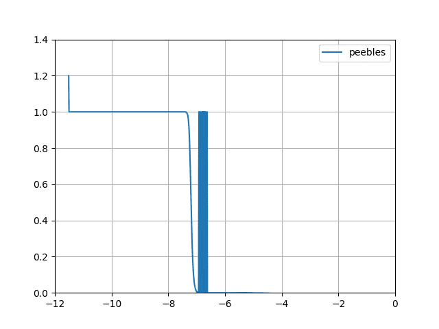
The graph I get is this

Can someone point out my mistake please? Or should I be using some other solver?
I have used both Runge Kutta 4th order and Radau IIA 5th order.

My initial conditions are:
a (scale factor) start (ts) = log(1e-5)
a end (tn) = log(1)
dt = (tn-ts)/1000

Xe = [1.2]

 

[Ibix]

Your program doesn't work for me. You haven't put in any actual call to fsolve. Guessing that this should be fsolve(fu, log(mpf('1e-5')), [mpf('1.2')]) causes the program to fail, complaining that it can't convert from an array to mpf in the first line of your fu function. Edit: and using that line and replacing all your mpf('x') with just x causes the program to fail complaining about a lack of convergence.

Also, you haven't labelled the axes on your graph so I have no idea what you're trying to plot.

Please post your complete program.

 

[Vick]

Your program doesn't work for me. You haven't put in any actual call to fsolve. Guessing that this should be fsolve(fu, log(mpf('1e-5')), [mpf('1.2')]) causes the program to fail, complaining that it can't convert from an array to mpf in the first line of your fu function. Edit: and using that line and replacing all your mpf('x') with just x causes the program to fail complaining about a lack of convergence.

Also, you haven't labelled the axes on your graph so I have no idea what you're trying to plot.

Please post your complete program.

My complete code includes the solvers for both RK4 and Radau5. However, if you are looking for my calling of it and the plotting thereof, here is the code:

ts = log(mpf('1e-5'))
tn = log(mpf('1'))
st = (tn-ts)/mpf('1000')
x = [mpf('1.2')]t=[]
a1=[]
for i in arange(ts, tn+st, st):
    t.append(i)
    a1.append(x)
   
    x = radau5(i,x,st)
   
import matplotlib.pyplot as plt
plt.figure()
plt.plot(t,a1, label='peebles')

plt.grid()
plt.axis([-12,0,0,1.4])
plt.legend()
plt.show()

I'm plotting scale factor 1e-5 to 1 as x-axis in log form and the Xe as y-axis; Xe[start] = 1.2

 

[Ibix]

Your new fragment doesn't call your fu function.

Unless you give us the complete program it's going to be almost impossible to help you with it. It's like going into a garage carrying an engine block and asking why your car doesn't run - at the moment it doesn't run because it isn't a car, it's just part of one.

 

[Vick]

Your new fragment doesn't call your fu function.

Unless you give us the complete program it's going to be almost impossible to help you with it. It's like going into a garage carrying an engine block and asking why your car doesn't run - at the moment it doesn't run because it isn't a car, it's just part of one.

def rungk4(t, x, dt):
    n = len(x)
    k1=[]; k2=[]; k3=[]; k4=[]; xcurr=[]; y=[]

    c2 = mpf('0.5')
    c3 = mpf('0.5')
    c4 = mpf('1')

    a21 = mpf('0.5')
    a31 = mpf('0')
    a32 = mpf('0.5')
    a41 = mpf('0')
    a42 = mpf('0')
    a43 = mpf('1')

    b1 = mpf('1.')/mpf('6')
    b2 = mpf('1.')/mpf('3')
    b3 = mpf('1.')/mpf('3')
    b4 = mpf('1.')/mpf('6')    a = fu(t,x)
    for i in range(n):
        k1.insert(i, dt * a[i])
        xcurr.insert(i, x[i] + \
                     k1[i] * a21)

    a = fu(t + dt * c2, xcurr)
    for i in range(n):
        k2.insert(i, dt * a[i])
        xcurr.insert(i, x[i] + \
                     k1[i] * a31 + \
                     k2[i] * a32)

    a = fu(t + dt * c3, xcurr)
    for i in range(n):
        k3.insert(i, dt * a[i])
        xcurr.insert(i, x[i] + \
                     k1[i] * a41 + \
                     k2[i] * a42 + \
                     k3[i] * a43)

    a = fu(t + dt * c4, xcurr)
    for i in range(n):
        k4.insert(i, dt * a[i])

    for i in range(n):
        y.insert(i, x[i] + (k1[i] * b1 + \
                            k2[i] * b2 + \
                            k3[i] * b3 + \
                            k4[i] * b4))

    return y

 

[Vick]

I have solved it. Is anyone interested or should I just close this thread?

 

[PeterDonis]

I have solved it.

If so, please post your solution.

 

[Vick]

The constants and imports are the same. However, I have modified the function itself for better debug and so I split it in several different ones.

I have also added the Saha Equation as shown in the article quoted above and also included reionization.

The necessary functions for Saha, Peebles and Reionization are as follows:

def sah(a):
    Tb = kb*cmbt/a
    np = (mpf('3')*h3**2*bdp)/ (mpf('8')*pi*g*mH*a**3)
    factor = ((mel*Tb)/(mpf('2')*pi*hp1**2))**(mpf('1.5'))/np

 
    fe  = mpf('1.0')
    fe_old = mpf('0.0')

   
    while (abs(fe-fe_old) > mpf('1.0e-10')):
       
        fac1 = 2.0*factor*exp(-xhi0/Tb)/fe
        fac2 = 4.0*factor*exp(-xhi1/Tb)/fe
        facH = factor*exp(-Ry/Tb)/fe

       
        x1 = fac1/(1.0 + fac1 + fac1*fac2)
        x2 = fac2 * x1
        xH = facH/(1.0 + facH)

        fe_old = fe
        fe = (2.0*x2+x1)*Yp/mpf('4.0') + (1.0-Yp)*xH
     

    Xe = fe/(1.0-Yp);
    ne = fe*np
   
    if (Xe < saha_limit):
        return 0, 0
    else:
        return Xe, ne
 def reion(a, Xe):
    fHe = Yp/(mpf('4')*(mpf('1')-Yp))
    yreion = (mpf('1') + zreion)**mpf('1.5')
    y = exp(-mpf('3')*a/mpf('2'))
    delyreion = mpf('1.5')*sqrt(mpf('1')+zreion)*delzreion
    rr = Xe[0] + (mpf('1')+fHe)/mpf('2')*(mpf('1')+tanh((yreion - y)/delyreion))+fHe/mpf('2')*(mpf('1')+tanh((zhereion-(exp(-a)-mpf('1')))/delzhereion))
    return rrdef H(a):
    return h3 * sqrt( (r * a ** mpf('-4'))
                      + (m * a ** mpf('-3'))
                      + (k * a ** mpf('-2'))
                      + l * exp(mpf('-6') * w1 * (mpf('1') - mpf('1')/ a)) / (a ** -(mpf('3') + mpf('3') * w0 + mpf('6') * w1)))def Tb(a):
    return kb*cmbt/adef nb(a):
    return (mpf('3')*h3**2*bdp)/ (mpf('8')*pi*g*mH*a**3)def o2Tb(a):
    return mpf('0.448')*ln(Ry/Tb(a))def a2Tb(a):
    return mpf('8')/sqrt(mpf('3')*pi) * sigmaT * sqrt(Ry/Tb(a))*o2Tb(a)def BTb(a):
    return a2Tb(a)*c*((mel*Tb(a))/(mpf('2')*pi*hp1**2))**(mpf('1.5')) * exp(-Ry/Tb(a))def delta(a, Xe):
    return ((mpf('1')-Xe[0])*BTb(a)/(c*nb(a)*a2Tb(a)*Xe[0]**2))def B2Tb(a):
    return BTb(a) * exp(mpf('0.75')*Ry/Tb(a))def n1s(a, Xe):
    return (mpf('1') - Xe[0])* (mpf('1')-Yp) * nb(a)def La(a, Xe):
    return H(a) * ((mpf('3')*Ry)**3)/((mpf('8')*pi)**2 * c**3 * hp1**3* n1s(a, Xe))def CrTb(a, Xe):
    L2s1s = mpf('8.227')
    return (L2s1s + La(a, Xe))/(L2s1s + La(a, Xe) + B2Tb(a))def fu(a, Xe):
    if delta(a, Xe) > mpf('1e-20'):
        return [CrTb(a, Xe)/H(a) *(BTb(a)*(1-Xe[0])-c*nb(a)*(mpf('1')-Yp)*a2Tb(a)*Xe[0]**2)]
    else:
        return [mpf('-1')/H(a)*c*nb(a)*(mpf('1')-Yp)*a2Tb(a)*Xe[0]**2]

I still used Runge Kutta 4th Order, albeit with a smaller delta t as shown below:

ts = mpf('-12')
tn = mpf('0')
st = (tn-ts)/mpf('100000')t1=[]; t2=[]

a1=[]; b1=[]; nel=[]; ree=[]; nee=[]

t3=[]; t4=[]for i in arange(ts, tn+st, st):
    x = sah(exp(i))
    if x[0] > saha_limit:
        t1.append(i)
        t3.append(exp(i))
        a1.append(x[0])
        nel.append(x[1])
    else:
        breakxx = [ a1[-1] ]
for i in arange(t1[-1], tn, st):
    t2.append(i+st)
    t4.append(exp(i+st))
    xx = rungk4(fu, exp(i), xx, st)
    b1.append(xx)
    x2s = reion(i, xx)
    ree.append(x2s)
    nee.append(x2s*(mpf('1')-Yp)*nb(exp(i+st)))

The first loop is for Saha and the second for Peebles and Reionization.

Please note that my code includes Helium as well, as per requirements of the article.

The final graph is as it should have been.