- #1
Dustinsfl
- 2,281
- 5
You can find problems with downloadable notebooks now http://www.mathhelpboards.com/f49/engineering-analysis-notes-2882/.
If one boundary is insulated and the other is subjected to and held at a temperature of unity, we wish to determine the solution for the transient heating of the slab.
The governing equation is the usual 1-D heat equation and the boundary conditions (mixed) are given by
\begin{alignat*}{3}
T_x(0,t) & = & 0\\
T(L,t) & = & 1
\end{alignat*}
with initial conditions
$$
T(x,0) = 0.
$$
Obtain the solution to this problem.
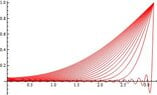
For the special case $\alpha = 1$ and $L = \pi$ plot a sequence of the temperature profiles between the initial state and the steady-state, construct a contour plot, density plot, and 3D plot.
Once we solve the problem, we obtain the solution as
$$
T(x,t) = 1 + \frac{4}{\pi}\sum_{n = 1}^{\infty}\frac{(-1)^n}{2n - 1}\cos\left[\left(n - \frac{1}{2}\right)x\right]\exp\left[-\left(n - \frac{1}{2}\right)^2t\right]
$$
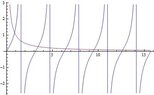
Next, we construct all the plots using Mathematica
This will produce the graph
https://www.physicsforums.com/attachments/390._xfImport
Adding in this piece of code will produce an animation between the different time profiles.
We can produce the contour plot by adding in
The end result is
https://www.physicsforums.com/attachments/393._xfImport
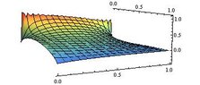
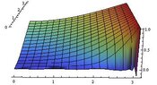
The density plot
The plot is
https://www.physicsforums.com/attachments/392._xfImport
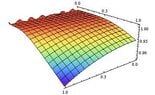
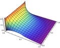
And lastly the 3d plot
https://www.physicsforums.com/attachments/391._xfImport
Here we can see the Gibbs Phenomenon occurring.
If one boundary is insulated and the other is subjected to and held at a temperature of unity, we wish to determine the solution for the transient heating of the slab.
The governing equation is the usual 1-D heat equation and the boundary conditions (mixed) are given by
\begin{alignat*}{3}
T_x(0,t) & = & 0\\
T(L,t) & = & 1
\end{alignat*}
with initial conditions
$$
T(x,0) = 0.
$$
Obtain the solution to this problem.
For the special case $\alpha = 1$ and $L = \pi$ plot a sequence of the temperature profiles between the initial state and the steady-state, construct a contour plot, density plot, and 3D plot.
Once we solve the problem, we obtain the solution as
$$
T(x,t) = 1 + \frac{4}{\pi}\sum_{n = 1}^{\infty}\frac{(-1)^n}{2n - 1}\cos\left[\left(n - \frac{1}{2}\right)x\right]\exp\left[-\left(n - \frac{1}{2}\right)^2t\right]
$$
Next, we construct all the plots using Mathematica
Code:
Nmax = 40;
L = Pi;
\[Lambda] = Table[(n - 1/2)*Pi/L, {n, 1, Nmax}];
\[Alpha] = 1;
MyTime = Table[t, {t, 0.0001, 1, .05}];
f[x_] = -1;

A = Table[2/L*Integrate[f[x]*Cos[\[Lambda][[n]]*x], {x, 0, L}], {n, 1,Nmax}];

u[x_, t_] = 1+Sum[A[[n]]*Cos[\[Lambda][[n]]*x]*E^{-\[Alpha]*\[Lambda][[n]]^2*t}, {n, 1, Nmax}];

Plot[u[x, MyTime], {x, 0, L}, PlotStyle -> {Red}]
This will produce the graph
https://www.physicsforums.com/attachments/390._xfImport
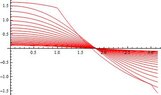
Adding in this piece of code will produce an animation between the different time profiles.
Code:
Animate[Plot[u[x, t], {x, 0, L}, PlotRange -> {0, 1.1}, GridLines -> Automatic, Frame -> True, PlotStyle -> {Thick, Red}], {t,0, 1, 0.02},
 AnimationRunning -> False]
Code:
ContourPlot[u[x, y], {x, 0, L}, {y, 0, L}, PlotRange -> All, ColorFunction -> "Rainbow"]The end result is
https://www.physicsforums.com/attachments/393._xfImport
The density plot
Code:
DensityPlot[u[x, y], {x, 0, L}, {y, 0, L}, PlotRange -> All, ColorFunction -> "Rainbow"]The plot is
https://www.physicsforums.com/attachments/392._xfImport
And lastly the 3d plot
Code:
Plot3D[u[x, y], {x, 0, L}, {y, 0, L}, PlotRange -> All, Boxed -> False, ColorFunction -> "Rainbow"]https://www.physicsforums.com/attachments/391._xfImport
Here we can see the Gibbs Phenomenon occurring.
Attachments


Last edited: