A Method for Proving Some Non-Linear Limits

[Ackbach]

I received permission from my father to post this from his (unpublished) Calculus text. Note that this method will, I believe, work for proving existence of a limit for a nonlinear function at any point that is not a local extremum. My father thought it would be good to give you this proviso before posting this.

... Up until this point, one might wonder whether
or not the entire aspect of limits isn't too easy. Well, let's us consider
a rather simple, but non-linear function such as $x^{2}$ and try to determine
the limit of this function as $x$ approaches $2$. Let us try the value of
$x^{2}$ itself at $x=2$ as the limit. In this case, it would mean trying $4$
for the limit. So, we would like to determine whether or not
$\lim x^{2}=4$ as $x\to 2$. The method we have tried so far is to set up
$|x^{2}-4|<\varepsilon$ and then squeeze the form $|x-2|<\delta$ from the $\varepsilon$
inequality. For our particular case, we start out with: $|x^{2}-4|<\varepsilon$
or $|(x-2)(x+2)|<\varepsilon$. This can be transformed to
$$|x-2|<\frac{\varepsilon}{|x+2|}.$$
So, we might think we can now simply let $\delta$ equal $\varepsilon/|x+2|$, and we
are again done with the problem?! Not so fast! If we do this, then $\delta$ is
a function not only of $\varepsilon$ but of $x$, and may or may not satisfy the
requirements for the limit. In order to make sure that we satisfy the
proper requirements for a limit, $\delta$ must be a function of $\varepsilon$
only, for the limit at anyone given point. Since this problem will come
up in all cases except for the linear function, we must find a method which
will work for these cases.

In general, for a non-linear function, the approach for verifying that the
limit of this function exists as $x$ approaches a given value boils down to
algebraically forcing $|f(x)-L|<\varepsilon$ into the form $|x-a|< \varepsilon|g(x)|$. Here,
of course, we have the problem of having $|g(x)|$ in the expression for what
we would like to represent as $\delta$.

So: what should we do? Well, a relatively simple approach would be this: why
not find a constant $\delta$ (say $\delta_{0}$) which will work for all
$ \varepsilon\ge \varepsilon_{0}$, and then use $\delta=c \varepsilon$ (where $c$ is a constant),
for all $ \varepsilon< \varepsilon_{0}$? (Remember, all we need to do is to find one
$\delta$ function which will work for all values of $ \varepsilon$; we do not
have to find the largest possible value for $\delta$ as a function of
$ \varepsilon$.) Therefore, the idea is to determine the proper value of $c$, the
constant $\delta_{0}$ good for large $ \varepsilon$, and we are finished with the
problem. We do have one option, which is to select our $ \varepsilon_{0}$. Once we do
that, $\delta_{0}$ can then be determined, and then finally the constant $c$.
To see how this is done, let us split the problem (of determining $\delta$)
into two parts:

• Find $\delta=\delta_{0}$ for $ \varepsilon\ge \varepsilon_{0}$.
  
  Suppose we have selected
  our $ \varepsilon_{0}$. Then we want $|f(x)-L|< \varepsilon_{0}$. This translates to the
  following:
  \begin{align*}
  - \varepsilon_{0}&<f(x)-L< \varepsilon_{0}\\
  \text{or,}\qquad L- \varepsilon_{0}&<f(x)<L+ \varepsilon_{0}
  \end{align*}
  
  If there is indeed a limit at $x=a$, then there must be a region
  $x_{1}<a<x_{2}$ such that $L- \varepsilon_{0}<f(x)<L+ \varepsilon_{0}$ whenever
  $x_{1}<x<x_{2}$. Consider the lesser of $a-x_{1}$ and $x_{2}-a$ and
  call it $\delta_{0}$. Then, as long as $|x-a|<\delta_{0}$, we will have:
  $-\delta_{0}<x-a<\delta_{0}$ or $a-\delta_{0}<x<\delta_{0}+a$, which will force
  $x$ to be between $x_{1}$ and $x_{2}$. But if $x$ lies between $x_{1}$ and
  $x_{2}$, then $L- \varepsilon_{0}<f(x)<L+ \varepsilon_{0}$, or $|f(x)-L|< \varepsilon_{0}$.
  Now for any $ \varepsilon\ge \varepsilon_{0}$, $ \varepsilon\ge \varepsilon_{0}>|f(x)-L|$, or
  $|f(x)-L|< \varepsilon$ for all $ \varepsilon\ge \varepsilon_{0}$. We have thus accomplished what we
  set out to do; namely, find a $\delta_{0}$, such that for all
  $|x-a|<\delta_{0}$, $|f(x)-L|< \varepsilon_{0}$ and also $|f(x)-L|< \varepsilon$ for all
  $ \varepsilon\ge \varepsilon_{0}$. The procedure for obtaining $\delta=\delta_{0}$, (which
  will work for all $ \varepsilon\ge \varepsilon_{0}$) is summarized as follows:
  1. Select an $ \varepsilon_{0}$ first
  2. Take $|f(x)-L|< \varepsilon_{0}$, work it algebraically to
     $L- \varepsilon_{0}<f(x)<L+ \varepsilon_{0}$, and finally work it down to $x_{1}<x<x_{2}$,
     where $x_{1}$ and $x_{2}$ will depend on $f(x)$, $L$, and the $ \varepsilon_{0}$ we
     pick.
  3. Take $\delta_{0}$ to be the lesser of $a-x_{1}$, and $x_{2}-a$.
  4. Then, for $|x-a|<\delta_{0}$, we know that $|f(x)-L|< \varepsilon$, for
     all $ \varepsilon\ge \varepsilon_{0}$.
  
  The next step is to obtain the value of the constant $c$, in $\delta=c \varepsilon$
  for all $ \varepsilon< \varepsilon_{0}$, which brings us to the second part of the problem:
• Find the constant $c$ for $\delta=c \varepsilon$, whenever $ \varepsilon< \varepsilon_{0}$.
  Here, as the title of this section suggests, we are going to try $\delta=c \varepsilon$.
  Recall that $|f(x)-L|< \varepsilon$ can, if a limit exists, be translated to the
  following: $|x-a|< \varepsilon|g(x)|$.
  
  Now, we are concerned about the situation where $|f(x)-L|< \varepsilon$ and
  $ \varepsilon< \varepsilon_{0}$. In this situation we naturally expect that $\delta$ will be
  less than $\delta_{0}$, which means that $x$ is between $a-\delta_{0}$
  and $a+\delta_{0}$. Now for $x$ restricted to such a region, we will have
  $|g(x)|$ bounded (i.e., it will be less than some positive number, as well
  as greater than zero). But, if $|g(x)|$ is greater than zero, it must have some
  minimum value $|g(x)|_{\min}$ over the region from $a-\delta_{0}$ to
  $a+\delta_{0}$. In many (if not most) of the cases we are dealing with, we
  shall find that $|g(x)|_{\min}$ occurs at an end point of the region
  $a-\delta_{0}$ to $a+\delta_{0}$. If such is not the case, then a
  selection of a smaller $\delta_{0}$, as outlined at the end of this
  section, may be necessary to ensure that $|g(x)|_{\min}$ occurs at the end
  of the interval $a-\delta_{0}$ to $a+\delta_{0}$. Let us suppose that
  $|g(x)|_{\min}$ does occur at one or the other end of the interval
  $a-\delta_{0}$ to $a+\delta_{0}$, for all $x$ in this interval. We then know
  that at one end we must have:
  $$
  \begin{aligned}
  |x-a|=\delta_{0}\\
  |f(x)-L|\le \varepsilon_{0}
  \end{aligned}
  \quad\text{from the previous section.}
  $$
  Also, because $|f(x)-L|< \varepsilon_{0}\to|x-a|< \varepsilon_{0}|g(x)|$, and because
  $g(x)=|g(x)|_{\min}$ at one end, $|x-a|$ at end
  $=\delta_{0}< \varepsilon_{0}|g(x)|_{\min}$. Therefore
  $\delta_{0}< \varepsilon_{0}|g(x)|_{\min}$ or
  $$\frac{\delta_{0}}{ \varepsilon_{0}}<|g(x)|_{\min}.$$
  Therefore, if we select $\delta$ such that:
  $|x-a|<\delta=\tfrac{\delta_{0}}{ \varepsilon_{0}}\, \varepsilon$, then because
  $\tfrac{\delta_{0}}{ \varepsilon_{0}}<|g(x)|_{\min}$, we have
  $|x-a|<\delta=\tfrac{\delta_{0}}{ \varepsilon_{0}}\, \varepsilon<|g(x)|_{\min}
  \varepsilon$.
  
  Therefore, if $|x-a|<\tfrac{\delta_{0}}{ \varepsilon_{0}}\, \varepsilon$, then
  $|x-a|< \varepsilon|g(x)|_{\min}$. But, $|g(x)|_{\min}<|g(x)|$ on the
  interval from $a-\delta_{0}$ to $a+\delta_{0}$. Whence:
  $|x-a|<\tfrac{\delta_{0}}{ \varepsilon_{0}}\, \varepsilon$ forces
  $|x-a|< \varepsilon|g(x)|_{\min}\le |g(x)| \varepsilon$, so that
  $|x-a|< \varepsilon|g(x)|$.
  
  But, $|x-a|< \varepsilon|g(x)|$ is the same thing as $|f(x)-L|< \varepsilon$.
  So, we have found our constant $c=\tfrac{\delta_{0}}{ \varepsilon_{0}}$,
  such that $|x-a|<c \varepsilon=\tfrac{\delta_{0}}{ \varepsilon_{0}}\, \varepsilon$
  will give $|f(x)-L|< \varepsilon$ for all $ \varepsilon< \varepsilon_{0}$. To summarize
  our method:
  1. Take the ratio of $\tfrac{\delta_{0}}{ \varepsilon_{0}}$, both of
     which were determined in the previous section.
  2. Check to verify that $|g(x)|$ is indeed a minimum at one
     of the two points $a-\delta_{0}$ and $a+\delta_{0}$.
  3. If 2. checks out, then set
     
     $\delta=\tfrac{\delta_{0}}{ \varepsilon_{0}}\, \varepsilon$ for all
     $ \varepsilon< \varepsilon_{0}$.
  
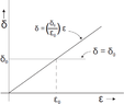
  Our final result: $\delta$ is $=\delta_{0}$ for $ \varepsilon> \varepsilon_{0}$
  
  and $\delta=\tfrac{\delta_{0}}{ \varepsilon_{0}}\, \varepsilon$ for
  
  $ \varepsilon< \varepsilon_{0}$. The graph of this is shown as follows:
  
  View attachment 728
  
  Note that in effect, $\delta$ is the lesser of
  $\left(\delta_{0},\tfrac{\delta_{0}}{ \varepsilon_{0}}\, \varepsilon\right)$.
  One final comment: If in step 2 of part B one finds that
  $|g(x)|_{\min}$ is not at $a-\delta_{0}$ or
  $a+\delta_{0}$, then select a smaller $ \varepsilon_{0}$ (call it
  $ \varepsilon_{0}'$) and go through the process of part A again.
  Afterwards, go through part B with the new $ \varepsilon_{0}'$ and
  $\delta_{0}'$, and check to see if $|g(x)|$ is a min on either
  $a-\delta_{0}'$ or $a+\delta_{0}'$, for $x$ lying in this new
  interval. As a rule, this process can be repeated until
  eventually one is successful in obtaining $|g(x)|_{\min}$ at
  the ends of a proper interval.

 

[Greg Bernhardt]

Thanks @Ackbach, what math forum can we move this to?

 

[Ackbach]

Thanks @Ackbach, what math forum can we move this to?

Math -> Calculus. This is good enough to sticky, I think.

 

[Svein]

Two forms of "limit" exist: pointwise limit and uniform limit.

 

[Ackbach]

Two forms of "limit" exist: pointwise limit and uniform limit.

Svein: Actually, there are loads of kinds of limits in various contexts. The context of this post is the pointwise limit $$\lim_{x\to a}f(x).$$

 

[Svein]

The context of this post is the pointwise limit

Yes, but that is the whole point of my answer. In an pointwise limit the δ in an ε - δ argument may very well depend on x. In a uniform limit argument, the δ is not allowed to depend on x.
A corollary: If a pointwise limit exists everywhere in a closed domain, it is also a uniform limit (take the maximum of all δ in the domain - if the domain is closed, the maximum exists).

 

[Ackbach]

Yes, but that is the whole point of my answer. In an pointwise limit the δ in an ε - δ argument may very well depend on x. In a uniform limit argument, the δ is not allowed to depend on x.
A corollary: If a pointwise limit exists everywhere in a closed domain, it is also a uniform limit (take the maximum of all δ in the domain - if the domain is closed, the maximum exists).

Agreed, but I'm not seeing where you're going with this. The proof technique above gives you a $\delta$ that is assuredly dependent on $x,$ even if it's implicit.