Bulk and Slab electronic structure differences

[MDT GH]

TL;DR

Calculate bulk and slab electronic structure with using DFT (Quantum ESPRESSO) has different results. Differences occur in calculating 𝜌𝜆 (i.e. figure of merit of thin film resistivity).

Hello dear.
I'm a graduate student specializing in Electronic Engineering.
This is my first question on this forum and I hope to get some advices in here.

I currently faced some challenges about DFT calculation.

My study is to analyze the low dimensional properties of metals.
And I try to figure it out by using the rho*lambda (ρ×λ, which refers resistivity and mean free path) factor.
I use Quantum ESPRESSO for DFT calculation, and use BolzTraP2 to get the ρ×λ from the DFT outputs.
*ρ×λ: resistivity×mean free path - figure of merit of thin metal film [1]

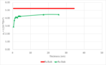
My thickness datas​

Slab structure​

I have been calculating the ρ×λ of metals at various thicknesses to find out the thickness dependence, and now I have a problem.
Well, I've tried to compare the resistivity of bulk and slab by using ρ×λ calculation (by using QE and BoltzTraP2[2]) and there I found slab's ρ×λ doesn't match with bulk value.
For example, ruthenium primitive cell, its ρ×λ property is 5.14*10^-16 [Ωm^2] in the paper [1] and I got 5.22*10^-16 [Ωm^2] from my BoltzTraP2.
But, while I make the system as a slab (i.g. add some 15 Angstrom vacuum along the Ru HCP 111 direction) its value comes out much smaller than the bulk after normalize, it has 2.9*10^-16 [Ωm^2].
I thought this because slab is too small to get the proper bulk characteristic, so I've also tried more larger size over 10~20 nm.
(the Ru has <10nm electron mean free path)
But in this size, the value is still small than bulk.
Also, they do not seem to match after increasing the size.

As far as I know, BoltzTraP2 doesn't have a relaxation time approximation, so it doesn't show the reduction in resistivity caused by surface scattering as the size scales. So I think they only have the electron band structure data, and these values leads some thickness dependence.

What can lead the thickness dependence in this situation?
Does slab and bulk has difference resistivity normal?

Thank you for all who read this question.
Best regards,
G. H.

[1] https://www.semanticscholar.org/pap...Gall/74143a843747e195369dfa89797e958e4b22de41
[2] https://arxiv.org/abs/1712.07946

 

[dRic2]

I agree that in the limit of thick slab contributions of the surface should impact less, thus, recovering the bulk value. You have a ~15 % relative error, it could be a convergence issue in the DFT. Did you check:
- convergence parameters (k-mesh,smearing,cutoff) both for the bulk and slab ?
- total energy per atom. Slab and Bulk values should approach each other in the thick limit, I believe.
It may be that you are running un-converged calculations.

 

[MDT GH]

Yes. I already tried to check both convergence many times.
But I did only with k-points.

1)
In my calculation, I set the 50x50x4 and 50x50x50 for each slab and bulk states.
And I'll share my results below.

<Convergence test>
Ru Slab with 4 unit cells along the c direction which means it has 8 atoms and 15 Angstrom vacuum along 'c' direction.

Tested by using NSCF data, based on SCF (15x15x1).
x axis is number of NSCF k-points along 'a', and 'b' direction which mean 10x10x4, 20x20x4, ... 60x60x4.

I choose 50x50x4 for right convergence of Ru slab.

Primitive cell convergence (Cu, I lost my data of Ru)

for bulk, the primitive cell, k-points set 50x50x50 (for NSCF, 15x15x15 for SCF)


2)
I use smearing option like below. [1]

• In input file, &SYSTEM
  occupations='smearing'
  starting_magnetization(1)= 1.0
  smearing='marzari-vanderbilt'
  degauss=0.02
• In &ELECTRONS
  mixing_beta = 0.1
  mixing_mode = 'local-TF'
  

3)
cutoff energy
I used the cutoff energy written in the pseudopotential file.
In Ru, the cutoff wave function is set as 52.0 [Ry] and the cutoff rho is set as 352.0 [Ry].

4)
Energy per atoms
I used 15x15x15 k-points for primitive Ru on SCF calculation,
and used 15x15x1 k-points for slab Ru on SCF calculation.

And I got each total energy and energy per atoms like below.

• Ru Primitive cell
  -863.34128250 / 2 = -431.6706413 [Ry]
• Ru Slab (x 4, which has 8 atoms and 3.2nm thickness)
  -3453.20670143 / 8 = -431.6508377 [Ry]
• Ru Slab (x 40. which has 80 atoms and 18.6nm thickness)
  -34533.49260269 / 80 = -431.6686575 [Ry]

Cu 111 plane (similar with HCP 001 direction)

• Cu Primitive cell - 111 plane (which has 3 Cu in the unit cell)
  -639.28267354 / 3 = -213.0942245 [Ry]
• Cu Slab (x1, which has 3 atoms and 2.1nm thickness)
  -639.2158504 / 3 = -213.0719501 [Ry]
• Cu Slab (x40, which has 120 atoms and 26.5nm thickness)
  -25571.23937 / 120 = -213.0936614 [Ry]

Thanks for your comment.
Please take a look my convergence tests and tell me something wrong.

Best regards,
G. H.

[1] QE pw.x input description (https://www.quantum-espresso.org/Doc/INPUT_PW.html)

 

[dRic2]

Sorry I don't quite follow your tests.

First of all, is your system magnetic?

About the convergence. Let's start with the SCF. How did you pick 15x15x1? And why those values for the smearing? Also the suggested value for cutoff seems to low in my opinion. Please also converge that value.
Note that you have to converge again for different systems (Cu and Ru could require different converged values).

In principle, what you do is the following:

- run SCF calculations for different values of psi_cutoff = 40,60,...,100,120,..., and rho _cutoff ~ 10*(psi_cutoff) and plot Total Energy vs cutoff. You should get a converging curve.
- repeat the process, but varying k-points and smearing. Plot Total Energy vs number of k-points for the different values of smearing, and again chose an appropriate value. 0.02 could be to low in my opinion.

Ideally you want an error on the total energy of the order of 1 meV.

About the input files, unless you know what you are doing, I recommend these settings:

occupations='smearing',
smearing='gauss',
degauss=*converged value*,

&electrons
diagonalization='davidson'
mixing_mode = 'plain'
mixing_beta = 0.7
conv_thr = 1.0d-9


Finally, you could try different pseudo potentials... but that should not be the case. These are the steps I always take before starting any calculations. I hope it might solve the issue.

 

[MDT GH]

Thank you for your kind explanation.

At first, my system, Ru doesn't have magnetic property.
Its total magnetization is -0.01 Bohr mag/cell after all iteration finished.

Well I'll try to figure out some other convergences, you guided,
but let me know first whether it reaches bulk property or not when the slab has sufficient thickness.

1) How did you pick 15x15x1?
I choose 15x15x1 because there is not quit big different between 15x15x 1~ 6 and also 20x20x1 or 30x30x1 (as I attached the fig on my previous reply).
Indeed, I tried to reduce the calculation time of scf as it use too much time on iteration.
So I allocate less k-points on scf, and more k-points on nscf.
After, the BoltzTraP2 use nscf data to interpolate and the converged rho*lambda comes out as like above.

2) About the input files, unless you know what you are doing, I recommend these settings

• smearing='marzari-vanderbilt' < don't know as well...
  I use this because they are much less dependent upon degauss and allow for faster and safer convergence than simple gaussian broadening [1] (watch on pp. 40-41)
• degauss = 0.02 < try
  Actually, I have no idea with the proper degauss before. And I set this value for the convergence speed for my bigger size calculation (more than 10~20 nm)
  I haven't been using *converged degauss value* before. Could you tell me where can I check it?

• diagonalization = 'davidson'
  This is an default option. I already use this :)
  so never mind.
• mixing_beta = 0.1 < try
  Also for bigger system convergence.
  But not quite important in Primitive and small cells.
  I usually set this value as default (a.k.a. 0.7). So it will be fine.
• mixing_mode = 'local-TF' < can't fix
  In slab system, which has inhomogeneous electron density, using local-TF is the best option for the convergence.
  Bigger system such over 10nm shouldn't converge as well without using this mode.
  
  
• conv_thr = 1.0d-6 < try
  Can you tell me why should I change minimum convergence threshold with 1.d-9 such more smaller than default?
  This may lead much calculation cost.
  Why I'd better not use the default?

My main question is that, does slab can approach the bulk value?
As I tested, the slab value seems saturated.

Best Regards,
G. H.

[1] https://gitlab.com/QEF/material-for.../master/Day-1/handson-day1.pdf?ref_type=heads

 

[dRic2]

My main question is that, does slab can approach the bulk value?

Yes it should, because surface contributions scales as $L^2$, while bulk as $L^3$, therefore in the thermodynamic limit ($L \rightarrow \infty$ they should not matter). That is why I am assuming calculations are not converged. Either that or the software has some problems.

from you post I see that k-mesh is well converged. Try converge rho and the smearing value. I saw the link you posted. In page 40-41 it is well explained all the convergence test that you should do. Follow the same steps and be sure the parameters are converged. (Convergence on rho is discussed a couple of page earlier)

Also if your system is not magnetic, don't make a magnetic calculation.

conv_thr = 1.0d-6 < try.
I don't know why it's the default value for you, but in my experience I have never used something less than 1.0d-9 (sometimes I went up to 10d-12). I am not using QE much recently, so I don't remember exactly why 1.0d-9. I guess depends on the types of calculations you need, but its seems that what you are doing requires quire precise band structure data, so I would set it higher.

mixing_mode = 'local-TF' < can't fix
I never used it. I found the original paper (https://www.researchgate.net/public...onsistency_in_density_functional_calculations) where this method is discussed and they say:

(The 'standard' mixing scheme) suffers from poor convergence
most noticeably when Eq. 1 is not solved to high accuracy for every SCF cycle

My understanding is that the standard mixing scheme is the best (https://www.vasp.at/wiki/index.php/Category:Density_mixing), you just need to be careful about convergence and use higher accuracy.

 

[MDT GH]

Thanks for your advice.

1)
At first, the reason I using
mixing_mode = 'local-TF'
is bad convergence of the plane mode.

When I using the mixing_mode = 'plane', scf iterations are hard to converge.
Some times they keep calculate over 300 steps and still not converged even I use mixing_beta = 0.1 (minimum value recommend? as I know), and more wide degauss.

Can you please tell my why the standard mixing scheme (perhaps plane mode?) is the best?
Sorry about my lack of knowledge.

2)
Second, magnetization.
Is there any problems occur after the magnetization calculation on non magnetic system?
Actually I checked the magnetization converged nearly 0 in the output file and I have no idea this gonna makes some difference whether we doing this calculation or not.
Additionally, I don't calculate spin no more. So the magnetization options will not affect now.

3)
Finally, ecutrho.
I'll gonna try this job henceforth.

Again, thanks for your mention.
Best regards,
G. H.