Determining the Max. Set of Linearly Independent Vectors

In summary, In "Principles of Quantum Mechanics" by R. Shankar, a vector space is defined as having dimension n if it can accommodate a maximum of n linearly independent vectors. The author attempts to prove that the set of all 2x2 matrices forms a four-dimensional vector space, using the fact that any arbitrary 2x2 matrix can be written in terms of four linearly independent vectors. However, this may not be obvious to students without prior knowledge of linear algebra. The author also cuts corners with the mathematical proofs in the book.
  • #1
DRose87
10
0
(sorry for the horrible butchered thread title... should say "determination", not "determining")
1. Homework Statement

In "Principles of Quantum Mechanics", by R. Shankar, a vector space is defined as having dimension n if it can accommodate a maximum of n linearly independent vectors (here is a free and legal preview of the math introduction. The parts I am discussing are on page 5 https://books.google.com/books?id=sDvrBwAAQBAJ&printsec=frontcover&source=gbs_ge_summary_r&cad=0#v=onepage&q&f=false). Immediately after this definition, the author attempts to prove that the set of all 2x2 matrices forms a four dimensional vector space. I am fully aware that this is the case, but the author's "proof" seems to be leaving out various facts, I think, needed to establish this (unless I am missing something and it should be completely obvious that 2x2 matrices can accommodate a maximum of n linearly independent vectors, without knowing anything of rules concerning spanning sets and bases, with have not been covered by this point in the book). The author states that because the matrices
Code:
[tex]\left| 1 \right\rangle  = \left[ {\begin{array}{*{20}{c}}
1&0\\
0&0
\end{array}} \right],\left| 2 \right\rangle  = \left[ {\begin{array}{*{20}{c}}
0&1\\
0&0
\end{array}} \right],\left| 3 \right\rangle  = \left[ {\begin{array}{*{20}{c}}
0&0\\
1&0
\end{array}} \right],\left| 4 \right\rangle  = \left[ {\begin{array}{*{20}{c}}
0&0\\
0&1
\end{array}} \right][/tex]
are linearly independent and since any arbitrary 2x2 matrix can be written in terms of them, it is impossible for 2x2 matrices with more than four matrices to be linearly independent. I understand that to be correct, and in a previous linear algebra course I remember proving that the maximum number of linearly independent vectors in a vector space is equal to the number of vectors in any basis for that space.

I just am wondering if this fact should be totally obvious, since the author just states that 2x2 matrices can accommodate at most four linearly independent vectors because any 2x2 matrix can be written as a combination of the four simple basis vectors shown above... before even mentioning what a basis is or explicitly stating why being able to write any 2x2 matrix as a combination of |1>,|2>,|3>,|4> prohibits the possible existence of five linearly independent vectors.

2 Attempt At A Solution
I looked in my notes and found a 'proof' (doubt a mathematician would say this is a valid proof but I'm satisfied with it :) ) that, if applied to a 2x2 vector space would show that it is of dimension 4... but it actually involved working out a lot of details lol... So I am wondering if the author of the book expects students to be familiar enough with linear algebra to know the results of the proof posted below... or if the fact that any set of 5 or more 2x2 matrices will be linearly dependent should be totally obvious considering that the basis posted above (which the author doesn't even call a basis... presumably up to this point in the book he hasn't even mentioned the concept of a basis) consists of four elements.
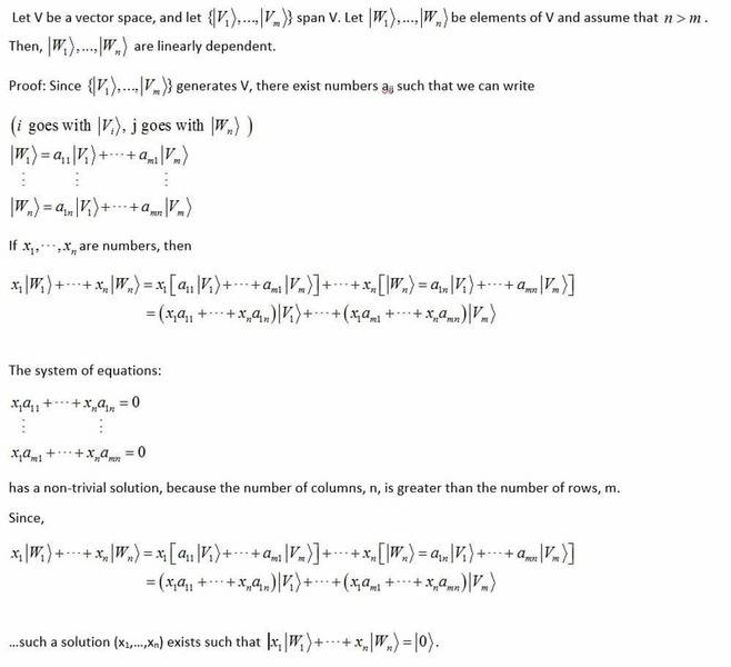
proof.jpg
 
Last edited:
Physics news on Phys.org
  • #2
You are right about Shankar. His book is good in many respects, but he does cut corners with his maths sometimes, and the one you have pointed to is such an occasion.

Re your proof. It all looks good except that the claim about the system of equations having a non-trivial solution is not obviously true (or not obvious enough for me at this time of night anyway). It sounds like a theorem from linear algebra. Is it one?
 
  • #3
andrewkirk said:
Re your proof. It all looks good except that the claim about the system of equations having a non-trivial solution is not obviously true (or not obvious enough for me at this time of night anyway). It sounds like a theorem from linear algebra. Is it one?
If the matrix form of the system of equations has more columns than rows, it might mean that there are non-trivial solutions, but it could mean that there are no solutions at all.

As an example, consider this system:
x + y + z = 1
x + y + z = 3

In matrix form this system is ##\begin{bmatrix} 1 & 1 & 1 \\ 1 & 1 & 1 \end{bmatrix}\begin{bmatrix} x \\ y\end{bmatrix} = \begin{bmatrix} 1 \\ 3\end{bmatrix}##
Using row reduction, it can be seen that there is no solution. Geometrically, the two equations represent two parallel planes with no points in common.
 
  • #4
Mark44 said:
it could mean that there are no solutions at all.
I think if the RHS of the equation is zero, there will always be at least one solution, being the one where ##\mathbf x## is the zero vector. So I suppose the theorem from linear algebra would need to be something like 'if ##A\mathbf x=0## and ##A## is a ##m\times n## matrix with ##n>m## and ##\mathbf x\in\mathbb R^n## then there exists at least one non-zero solution to the equation.' I am wondering whether it needs to also say something about column or row rank, but perhaps not.
 
  • #5
andrewkirk said:
You are right about Shankar. His book is good in many respects, but he does cut corners with his maths sometimes, and the one you have pointed to is such an occasion.

Re your proof. It all looks good except that the claim about the system of equations having a non-trivial solution is not obviously true (or not obvious enough for me at this time of night anyway). It sounds like a theorem from linear algebra. Is it one?
Thanks. Yeah I pretty much just blew past that without giving an explanation because it was something I learned in linear algebra, and the reason it is true seems pretty obvious to me at this point.

Here is not a real 'proof', but I think an explanation that should make the truth of that statement seem pretty clear.
Obviously any system of m linear equations with n unknowns, with each equation equal to 0, has at least one solution (each of the unknowns is equal to 0). But... if a system of m equations in n unknowns, with each equation equal to 0, has more unknowns, n, then equations, there must be at least one non-trivial solution... and therefore there will be an infinite number of solutions (since any multiply of a non-trivial solution give you another non-trivial solution).

If you've studied linear algebra I assume you've learned about row reduction, row echelon form and reduced row echelon form... and in particular how when you do row reduction on a system of linear equations, the row reduced system that you end up with after reduction is 'row equivalent' to the original system, which basically just means that the system you start out with and the system you end up with have identical solution sets.

If you have a system of m linear equations in n unknowns, with each equation equal to 0, and if n > m, it is pretty easy to demonstrate that the system must have at least one non-trivial solution (and therefore an infinite number of non-trivial solutions)

When you perform row reduction, the most "pivots" (a pivot being the first non-zero element in a row) that you can end up with is m, since their are m rows. Assuming you have m pivots, which is the max number of pivots, and using a system with 3 equations in 4 unknowns as an example, you'll end up with a row echelon system with n-m>0 "free variables"... in other words, if n>m (more variables then equations), you'll end up with at least one free variable, which is a variable that you can give any value you want and get, through back substitution, a solution to the system. (If you have m equation in n unknowns, and each equation is equal to 0, if you end up with r pivots after row reduction, you will get r-n free variables). This is pretty clear if you break the system down further into reduced-row echelon form (1's in the pivot positions, 0's above an below pivots).

Code:
[tex]\begin{array}{l}
\left[ {\begin{array}{*{20}{c}}
1&0&0&{{a_{14}}}\\
0&1&0&{{a_{24}}}\\
0&0&1&{{a_{34}}}
\end{array}} \right] \to \left[ {\begin{array}{*{20}{c}}
1&0&0&{{a_{14}}}\\
0&1&0&{{a_{24}}}\\
0&0&1&{{a_{34}}}
\end{array}} \right]\underbrace {\left[ {\begin{array}{*{20}{c}}
{{x_1}}\\
{{x_2}}\\
{{x_3}}\\
{{x_4}}
\end{array}} \right]}_x{\rm{ =  }}\left[ {\begin{array}{*{20}{c}}
{{x_1} + {a_{14}}{x_4}}\\
{{x_2} + {a_{24}}{x_4}}\\
{{x_3} + {a_{34}}{x_4}}
\end{array}} \right]{\rm{ = }}\left[ {\begin{array}{*{20}{c}}
0\\
0\\
0
\end{array}} \right]\\
{\rm{   }}\\
{x_3} =  - {a_{34}}{x_4}\\
{x_2} =  - {a_{24}}{x_4}\\
{x_1} =  - {a_{14}}{x_4}\\
\\
x = \left[ {\begin{array}{*{20}{c}}
{{x_1}}\\
{{x_2}}\\
{{x_3}}\\
{{x_4}}
\end{array}} \right] = \left[ {\begin{array}{*{20}{c}}
{ - {a_{14}}}\\
{ - {a_{24}}}\\
{ - {a_{34}}}\\
1
\end{array}} \right]{x_4}
\end{array}[/tex]

If the system has just 2 pivots... it might look like this...
Code:
[tex]\begin{array}{l}
\left[ {\begin{array}{*{20}{c}}
1&0&0&{{a_{14}}}\\
0&1&{{a_{23}}}&{{a_{24}}}\\
0&0&0&0
\end{array}} \right] \to \left[ {\begin{array}{*{20}{c}}
1&0&{{a_{13}}}&{{a_{14}}}\\
0&1&{{a_{23}}}&{{a_{24}}}\\
0&0&0&0
\end{array}} \right]\underbrace {\left[ {\begin{array}{*{20}{c}}
{{x_1}}\\
{{x_2}}\\
{{x_3}}\\
{{x_4}}
\end{array}} \right]}_x{\rm{ =  }}\left[ {\begin{array}{*{20}{c}}
{{x_1} + {a_{13}}{x_3} + {a_{14}}{x_4}}\\
{{x_2} + {a_{23}}{x_3} + {a_{24}}{x_4}}\\
0
\end{array}} \right]{\rm{ = }}\left[ {\begin{array}{*{20}{c}}
0\\
0\\
0
\end{array}} \right]\\
{\rm{   }}\\
{x_2} =  - {a_{23}}{x_3} +  - {a_{24}}{x_4}\\
{x_1} =  - {a_{13}}{x_3} +  - {a_{14}}{x_4}\\
\underbrace {\left[ {\begin{array}{*{20}{c}}
{{x_1}}\\
{{x_2}}\\
{{x_3}}\\
{{x_4}}
\end{array}} \right]}_x = \left[ {\begin{array}{*{20}{c}}
{ - {a_{13}}}\\
{ - {a_{23}}}\\
1\\
0
\end{array}} \right]{x_3} + \left[ {\begin{array}{*{20}{c}}
{ - {a_{14}}}\\
{ - {a_{24}}}\\
1\\
0
\end{array}} \right]{x_x}
\end{array}[/tex]

And with just 1 pivot... assuming the pivot is in the first column...which doesn't really matter...
Code:
[tex]\begin{array}{l}
\left[ {\begin{array}{*{20}{c}}
1&0&0&{{a_{14}}}\\
0&0&0&0\\
0&0&0&0
\end{array}} \right] \to \left[ {\begin{array}{*{20}{c}}
1&{{a_{12}}}&{{a_{13}}}&{{a_{14}}}\\
0&0&0&0\\
0&0&0&0
\end{array}} \right]\underbrace {\left[ {\begin{array}{*{20}{c}}
{{x_1}}\\
{{x_2}}\\
{{x_3}}\\
{{x_4}}
\end{array}} \right]}_x{\rm{ =  }}\left[ {\begin{array}{*{20}{c}}
{{x_1} + {a_{12}}{x_2} + {a_{13}}{x_3} + {a_{14}}{x_4}}\\
0\\
0
\end{array}} \right]{\rm{ = }}\left[ {\begin{array}{*{20}{c}}
0\\
0\\
0
\end{array}} \right]\\
{\rm{   }}\\
{x_1} =  - {a_{12}}{x_2} - {a_{13}}{x_3} +  - {a_{14}}{x_4}\\
\underbrace {\left[ {\begin{array}{*{20}{c}}
{{x_1}}\\
{{x_2}}\\
{{x_3}}\\
{{x_4}}
\end{array}} \right]}_x = \left[ {\begin{array}{*{20}{c}}
{ - {a_{12}}}\\
1\\
0\\
0
\end{array}} \right]{x_2} + \left[ {\begin{array}{*{20}{c}}
{ - {a_{13}}}\\
0\\
1\\
0
\end{array}} \right]{x_3} + \left[ {\begin{array}{*{20}{c}}
{ - {a_{14}}}\\
0\\
0\\
1
\end{array}} \right]{x_4}
\end{array}[/tex]

A random example...
Code:
[tex]\begin{array}{l}
3{x_1} + 4{x_2} + 5{x_3} = 0\\
9{x_1} + 6{x_2} + 3{x_3} = 0\\
\left[ {\begin{array}{*{20}{c}}
2&4&1\\
4&6&3
\end{array}} \right]\left[ {\begin{array}{*{20}{c}}
{{x_1}}\\
{{x_2}}\\
{{x_3}}
\end{array}} \right] = \left[ {\begin{array}{*{20}{c}}
0\\
0\\
0
\end{array}} \right]\\
\left[ {\begin{array}{*{20}{c}}
2&4&1\\
4&6&3
\end{array}} \right] \to \left[ {\begin{array}{*{20}{c}}
2&4&1\\
{4 - 2\left( 2 \right)}&{6 - 2\left( 4 \right)}&{3 - \left( {2 \cdot 1} \right)}
\end{array}} \right] = \left[ {\begin{array}{*{20}{c}}
2&4&1\\
0&{ - 2}&1
\end{array}} \right]\\
\to \left[ {\begin{array}{*{20}{c}}
{2 + \left( {2 \cdot 0} \right)}&{4 + \left( {2 \cdot  - 2} \right)}&{1 + \left( {2 \cdot 1} \right)}\\
0&{ - 2}&1
\end{array}} \right] = \left[ {\begin{array}{*{20}{c}}
2&0&3\\
0&{ - 2}&1
\end{array}} \right]\\
\to \left[ {\begin{array}{*{20}{c}}
{2/2}&0&{3/2}\\
0&{ - 2/ - 2}&{1/ - 2}
\end{array}} \right] = \left[ {\begin{array}{*{20}{c}}
1&0&{3/2}\\
0&1&{ - 1/2}
\end{array}} \right]\\
\\
\left[ {\begin{array}{*{20}{c}}
1&0&{3/2}\\
0&1&{ - 1/2}
\end{array}} \right]\left[ {\begin{array}{*{20}{c}}
{{x_1}}\\
{{x_2}}\\
{{x_3}}
\end{array}} \right] = \left[ {\begin{array}{*{20}{c}}
0\\
0\\
0
\end{array}} \right] = \left[ {\begin{array}{*{20}{c}}
{{x_1} + \frac{3}{2}{x_3}}\\
{{x_2} - \frac{1}{2}{x_3}}\\
0
\end{array}} \right]\\
{x_2} - \frac{1}{2}{x_3} = 0 \to {x_2} = \frac{1}{2}{x_3}\\
{x_1} + \frac{3}{2}{x_3} = 0 \to {x_1} =  - \frac{3}{2}{x_3}\\
\\
\left[ {\begin{array}{*{20}{c}}
{{x_1}}\\
{{x_2}}\\
{{x_3}}
\end{array}} \right] = \left[ {\begin{array}{*{20}{c}}
{\frac{1}{2}{x_3}}\\
{ - \frac{3}{2}{x_3}}\\
{{x_3}}
\end{array}} \right] = \left[ {\begin{array}{*{20}{c}}
{\frac{1}{2}}\\
{ - \frac{3}{2}}\\
1
\end{array}} \right]{x_3}\\

\end{array}[/tex]
 
Last edited:
  • #6
andrewkirk said:
I think if the RHS of the equation is zero, there will always be at least one solution, being the one where ##\mathbf x## is the zero vector. So I suppose the theorem from linear algebra would need to be something like 'if ##A\mathbf x=0## and ##A## is a ##m\times n## matrix with ##n>m## and ##\mathbf x\in\mathbb R^n## then there exists at least one non-zero solution to the equation.' I am wondering whether it needs to also say something about column or row rank, but perhaps not.

Basically the only way that a system of equations all equal to zero will only have the trivial solution is if its rank (the number of pivot columns) is equal to the number of columns of the matrix. In that case, in reduced row echelon form, you would have 1's in the pivot positions... there would be a pivot in every column... and since for row reduced row echelon form you have 0's above and below the pivots... each column would have all 0's except for in the pivot position... if you had a square matrix, the reduced-row echelon form of a system with a pivot in each column would just be the identity matrix.

Example:
Code:
[tex]\begin{array}{l}

{x_1} + 2{x_2} + 4{x_3} = 0\\
2{x_2} + 4{x_2} + 8{x_3} = 0\\
3{x_2} + 6{x_2} + 12{x_3} = 0\\
\left[ {\begin{array}{*{20}{c}}
1&2&4\\
2&5&8\\
3&7&{13}
\end{array}} \right] \to \left[ {\begin{array}{*{20}{c}}
1&2&4\\
0&1&0\\
0&1&1
\end{array}} \right] \to \left[ {\begin{array}{*{20}{c}}
1&2&4\\
0&1&0\\
0&0&1
\end{array}} \right]
\end{array}[/tex]
We could just stop here at row echelon form without getting to reduced row echelon form and do back substitution from here to see why this will only have the trivial solution.

[tex]\begin{array}{l}
{x_1} + 2{x_2} + 4{x_3} = 0\\
2{x_2} + 5{x_2} + 8{x_3} = 0\\
3{x_2} + 7{x_2} + 13{x_3} = 0\\
\left[ {\begin{array}{*{20}{c}}
1&2&4\\
2&5&8\\
3&7&{13}
\end{array}} \right] \to \left[ {\begin{array}{*{20}{c}}
1&2&4\\
0&1&0\\
0&1&1
\end{array}} \right] \to \left[ {\begin{array}{*{20}{c}}
1&2&4\\
0&1&0\\
0&0&1
\end{array}} \right]\\
\\
\left[ {\begin{array}{*{20}{c}}
1&2&4\\
0&1&0\\
0&0&1
\end{array}} \right]\left[ {\begin{array}{*{20}{c}}
{{x_1}}\\
{{x_2}}\\
{{x_3}}
\end{array}} \right] = \left[ {\begin{array}{*{20}{c}}
0\\
0\\
0
\end{array}} \right]\\
{x_3} = 0\\
{x_2} = 0\\
{x_1} + 2{x_2} + 4{x_3} = 0 \to {x_1} = - 2{x_2} + - 4{x_3} = - 2\left( 0 \right) + - 4\left( 0 \right) = 0\\
x = \left[ {\begin{array}{*{20}{c}}
0\\
0\\
0
\end{array}} \right]
\end{array}[/tex]If we had two or fewer pivots, we'd have infinity many trivial solutions.
[tex]\begin{array}{l}
{x_1} + 2{x_2} + 4{x_3} = 0\\
2{x_2} + 5{x_2} + 9{x_3} = 0\\
3{x_2} + 6{x_2} + 12{x_3} = 0\\
\left[ {\begin{array}{*{20}{c}}
1&2&4\\
2&5&9\\
3&6&{12}
\end{array}} \right] \to \left[ {\begin{array}{*{20}{c}}
1&2&4\\
0&1&1\\
0&0&0
\end{array}} \right]\\
\\
\left[ {\begin{array}{*{20}{c}}
1&2&4\\
0&1&1\\
0&0&0
\end{array}} \right]\left[ {\begin{array}{*{20}{c}}
{{x_1}}\\
{{x_2}}\\
{{x_3}}
\end{array}} \right] = \left[ {\begin{array}{*{20}{c}}
0\\
0\\
0
\end{array}} \right]\\
{x_2} + {x_3} = 0 \to {x_2} = - {x_3}\\
{x_1} + 2{x_2} + 4{x_3} = 0 \to {x_1} = - 2{x_2} - 4{x_3} = 2{x_3} - 4{x_3} = - 2{x_3}\\
\\
x = \left[ {\begin{array}{*{20}{c}}
{{x_1}}\\
{{x_2}}\\
{{x_3}}
\end{array}} \right] = \left[ {\begin{array}{*{20}{c}}
{ - 2{x_3}}\\
{ - {x_3}}\\
{{x_3}}
\end{array}} \right] = \left[ {\begin{array}{*{20}{c}}
{ - 2}\\
{ - 1}\\
1
\end{array}} \right]{x_3}
\end{array}[/tex]

If the number of rows is greater than the number of columns, it is still possible to have only a trivial solution, since you could still have a pivot in every column.

Example:
[tex]\begin{array}{l}
\left[ {\begin{array}{*{20}{c}}
1&4\\
1&9\\
2&0
\end{array}} \right] \to \left[ {\begin{array}{*{20}{c}}
1&8\\
0&5\\
0&{ - 8}
\end{array}} \right] \to \left[ {\begin{array}{*{20}{c}}
1&8\\
0&5\\
0&0
\end{array}} \right] \to \left[ {\begin{array}{*{20}{c}}
1&8\\
0&1\\
0&0
\end{array}} \right] \to \left[ {\begin{array}{*{20}{c}}
1&0\\
0&1\\
0&0
\end{array}} \right]\\
{x_1} = 0\\
{x_2} = 0
\end{array}[/tex]

...

This should cover every possible scenario for systems given by Ax=0, with A being m x n (not proofs... but explanations)

If m = n (n equations in m unknowns), the system has a non-trivial solution (and therefore an infinite number of non-trivial solutions) if and only if its rank equals n, meaning it has n pivots (reduced row echelon form being the n x n identity matrix). If you have less than n pivots, you will have at least 1 'free variable', corresponding to one of the components of x. If m > n, (m equations in n unknowns), the system has a non-trivial solution (and therefore an infinite number of non-trivial solutions) if and only if its rank equals n, the number of columns. Its reduced-row echelon form matrix will have 1's in the pivot positions, and 0's above and below each pivot. The pivot in column 1 corresponds to x1, the pivot in column 2 corresponds to x2, etc. Therefore you'd get x1=0,x2=0,etc.
If n > m. If you have less than n pivots, you'd have at least 1 free variable.

If n > m, you will have an infinite number of non-trivial solutions, because you can have at most m pivots, so at least one column won't contain a pivot.
 
Last edited:
  • #7
Gilbert Strang, in his book "Differential Equations and Linear Algebra" has a pretty simple proof that every basis of a particular vector space has the same number of vectors. A basis for a vector space is a sequence of vectors that are linearly independent and span the space.

If {w1,...,wn} and {u1,...,un} are a basis, each of the w's must be a linear combination of the u's.
[tex]{\rm{If \ }}{{\bf{w}}_i} = {a_1}_i{{\bf{u}}_1} + ... + {a_{mi}}{{\bf{u}}_m}[/tex], this is the ith column of a matrix multiplication.
Let
[tex]W = \left[ {\begin{array}{*{20}{c}}
{{{\bf{w}}_1}}&{{{\bf{w}}_2}}&{...}&{{{\bf{w}}_n}}
\end{array}} \right],U = \left[ {\begin{array}{*{20}{c}}
{{{\bf{u}}_{\bf{1}}}}&{...}&{{{\bf{u}}_m}}
\end{array}} \right],A = \left[ {\begin{array}{*{20}{c}}
{{a_{11}}}& \cdots &{{a_{1n}}}\\
\vdots & \vdots & \vdots \\
{{a_{m1}}}& \cdots &{{a_{mn}}}
\end{array}} \right][/tex]

It follows that
[tex]W = \left[ {\begin{array}{*{20}{c}}
{{{\bf{w}}_1}}&{{{\bf{w}}_2}}&{...}&{{{\bf{w}}_n}}
\end{array}} \right] = \left[ {\begin{array}{*{20}{c}}
{{{\bf{u}}_{\bf{1}}}}&{...}&{{{\bf{u}}_m}}
\end{array}} \right]\left[ {\begin{array}{*{20}{c}}
{{a_{11}}}& \cdots &{{a_{1n}}}\\
\vdots & \vdots & \vdots \\
{{a_{m1}}}& \cdots &{{a_{mn}}}
\end{array}} \right] = UA[/tex]

[tex]{{\rm{column \ i \ of \ W}} = {w_i} = U \cdot {\rm{\ column \ i \ of \ A}}}[/tex]

Since A is an mxn matrix, there must be at least one
[tex]{\bf{v}} = \left[ {\begin{array}{*{20}{c}}
{{v_1}}\\
\vdots \\
{{v_n}}
\end{array}} \right] \ne {\bf{0}}[/tex]
such that
[tex]A{\bf{v}} = \left[ {\begin{array}{*{20}{c}}
{{a_{11}}}&{}&{{a_{1n}}}\\
\vdots &{}& \vdots \\
{{a_{m1}}}&{}&{{a_{mn}}}
\end{array}} \right]\left[ {\begin{array}{*{20}{c}}
{{v_1}}\\
\vdots \\
{{v_n}}
\end{array}} \right] = {\bf{0}}[/tex]

and
[tex]W{\bf{v}} = \left[ {\begin{array}{*{20}{c}}
{{{\bf{w}}_{\bf{1}}}}&{{{\bf{w}}_{\bf{2}}}}&{...}&{{{\bf{w}}_{\bf{n}}}}
\end{array}} \right]\left[ {\begin{array}{*{20}{c}}
{{v_1}}\\
{{v_2}}\\
\vdots \\
{{v_3}}
\end{array}} \right] = \left[ {\begin{array}{*{20}{c}}
{{{\bf{u}}_{\bf{1}}}}&{...}&{{{\bf{u}}_m}}
\end{array}} \right]\left[ {\begin{array}{*{20}{c}}
{{a_{11}}}&{}&{{a_{1n}}}\\
\vdots &{}& \vdots \\
{{a_{m1}}}&{}&{{a_{mn}}}
\end{array}} \right]\left[ {\begin{array}{*{20}{c}}
{{v_1}}\\
\vdots \\
{{v_n}}
\end{array}} \right] = \left[ {\begin{array}{*{20}{c}}
{{u_1}}&{...}&{{u_m}}
\end{array}} \right]{\bf{0}} = {\bf{0}}[/tex]

Therefore, a non-trivial combination of the w's gives 0, so the w's cannot be a basis (they are linearly dependent). The assumption that n>m is not possible for two basis. If m>n we u's and w's and repeat the same steps. The only way to avoid a contradiction is if m=n.
 
  • #8
DRose87 said:
(sorry for the horrible butchered thread title... should say "determination", not "determining")
1. Homework Statement

In "Principles of Quantum Mechanics", by R. Shankar, a vector space is defined as having dimension n if it can accommodate a maximum of n linearly independent vectors (here is a free and legal preview of the math introduction. The parts I am discussing are on page 5 https://books.google.com/books?id=sDvrBwAAQBAJ&printsec=frontcover&source=gbs_ge_summary_r&cad=0#v=onepage&q&f=false). Immediately after this definition, the author attempts to prove that the set of all 2x2 matrices forms a four dimensional vector space. I am fully aware that this is the case, but the author's "proof" seems to be leaving out various facts, I think, needed to establish this (unless I am missing something and it should be completely obvious that 2x2 matrices can accommodate a maximum of n linearly independent vectors, without knowing anything of rules concerning spanning sets and bases, with have not been covered by this point in the book). The author states that because the matrices
Code:
[tex]\left| 1 \right\rangle  = \left[ {\begin{array}{*{20}{c}}
1&0\\
0&0
\end{array}} \right],\left| 2 \right\rangle  = \left[ {\begin{array}{*{20}{c}}
0&1\\
0&0
\end{array}} \right],\left| 3 \right\rangle  = \left[ {\begin{array}{*{20}{c}}
0&0\\
1&0
\end{array}} \right],\left| 4 \right\rangle  = \left[ {\begin{array}{*{20}{c}}
0&0\\
0&1
\end{array}} \right][/tex]
are linearly independent and since any arbitrary 2x2 matrix can be written in terms of them, it is impossible for 2x2 matrices with more than four matrices to be linearly independent. I understand that to be correct, and in a previous linear algebra course I remember proving that the maximum number of linearly independent vectors in a vector space is equal to the number of vectors in any basis for that space.

I just am wondering if this fact should be totally obvious, since the author just states that 2x2 matrices can accommodate at most four linearly independent vectors because any 2x2 matrix can be written as a combination of the four simple basis vectors shown above... before even mentioning what a basis is or explicitly stating why being able to write any 2x2 matrix as a combination of |1>,|2>,|3>,|4> prohibits the possible existence of five linearly independent vectors.

2 Attempt At A Solution
I looked in my notes and found a 'proof' (doubt a mathematician would say this is a valid proof but I'm satisfied with it :) ) that, if applied to a 2x2 vector space would show that it is of dimension 4... but it actually involved working out a lot of details lol... So I am wondering if the author of the book expects students to be familiar enough with linear algebra to know the results of the proof posted below... or if the fact that any set of 5 or more 2x2 matrices will be linearly dependent should be totally obvious considering that the basis posted above (which the author doesn't even call a basis... presumably up to this point in the book he hasn't even mentioned the concept of a basis) consists of four elements.

proof.jpg

Back in the Stone Age when I took Linear Algebra, we had a simple proof that in a finite-dimensional vector space, all bases consist of equal numbers of vectors.

To see this, let ##{\cal V} = \{v_1, v_2, \ldots, v_n\}## and ##{\cal W} = \{w_1, w_2, \ldots, w_m\}## be two bases, with ##m \geq n##. Since ##w_1## is a non-trivial linear combination of the ##v_i##, we can write ##w_1 = c_1 v_1 + c_2 v_2 + \cdots + c_n v_n##, with ##c_1 \neq 0## (by re-labelling the ##v_j## if necessary). Thus, we have
$$v_1 = \frac{1}{c_1} w_1 - \frac{c_2}{c_1} v_2 -\cdots \frac{c_n}{c_1} v_n$$
It follows that ##{\cal V}_1 = \{ w_1, v_2, v_3, \ldots, v_n \}## is a basis.

Using the fact that ##{\cal V}_1## and ##{\cal W}## are bases, we can argue similarly that ##{\cal V}_2 = \{ w_1, w_2, v_3, \ldots, v_n \}## is a basis. Keep going like that, swapping ##w_j## for ##v_j##, until all ##n## of the ##v_i## have been "used up". That means that ##{\cal V}_n = \{w_1, w_2, \ldots, w_n \}## is a basis, and so we cannot have ##m > n##.

This argument leaves out some details, but these missing ingredients are not overly challenging.
 
Last edited:

What is the purpose of determining the maximum set of linearly independent vectors?

The purpose of determining the maximum set of linearly independent vectors is to find a basis for a vector space. This basis will consist of a set of vectors that are linearly independent, meaning no vector can be expressed as a linear combination of the other vectors in the set. This is important in various mathematical and scientific applications, such as solving systems of equations, finding eigenvalues and eigenvectors, and performing transformations.

How do you determine the maximum set of linearly independent vectors?

To determine the maximum set of linearly independent vectors, you can use the Gaussian elimination method. This involves creating a matrix from the given set of vectors and performing row operations to reduce the matrix to row-echelon form. The number of non-zero rows in the reduced matrix will give you the maximum number of linearly independent vectors.

What is the difference between linearly independent and linearly dependent vectors?

Linearly independent vectors are those that cannot be expressed as a linear combination of the other vectors in the set. In other words, they are not redundant and provide unique information. On the other hand, linearly dependent vectors are those that can be written as a linear combination of the other vectors in the set. This means they are not necessary in the set and can be removed without losing any information.

Can a set of vectors have more than one maximum set of linearly independent vectors?

No, a set of vectors can only have one maximum set of linearly independent vectors. This is because the maximum number of linearly independent vectors is equal to the dimension of the vector space. Any additional vectors would result in a linearly dependent set, which goes against the definition of maximum set of linearly independent vectors.

What is the significance of a maximum set of linearly independent vectors in linear algebra?

In linear algebra, a maximum set of linearly independent vectors is significant because it forms a basis for the vector space. This basis is essential in solving systems of equations, finding eigenvalues and eigenvectors, and performing transformations. Additionally, it allows for efficient and accurate computations when dealing with large sets of data.

Similar threads

  • Calculus and Beyond Homework Help
Replies
18
Views
1K
  • Calculus and Beyond Homework Help
Replies
2
Views
984
  • Calculus and Beyond Homework Help
Replies
14
Views
592
  • Calculus and Beyond Homework Help
Replies
1
Views
278
  • Calculus and Beyond Homework Help
Replies
15
Views
2K
  • Calculus and Beyond Homework Help
Replies
6
Views
532
  • Calculus and Beyond Homework Help
Replies
0
Views
449
  • Calculus and Beyond Homework Help
Replies
4
Views
1K
  • Calculus and Beyond Homework Help
Replies
10
Views
1K
  • Calculus and Beyond Homework Help
Replies
0
Views
151
Back
Top