Generate heat conduction curves at different time steps

[SimoneSk]

Dear all,
I am having some difficulties in generating some heat conduction curves.
My problem is:
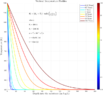
I have an object at a temperature (Th) of 900 K placed on top of a surface with a temperature (Ta) of 300 K (see Figure). The thermal conductivity (K; W M-1 K-1) is 1.5 whilst the thermal diffusivity (a; m2 s-1) is 7e-07.
I would like to apply a 1-D heat conduction model that would show the temperature profile with depth after 1 second, 1 minute, 1 hour, 12 hours, 1 day, 2 days, 10 days, and 365 days.
The output would ideally look something like:

Would you kindly be able to suggest what approach best applies to my problem? Are the information provided sufficient to solve the problem?
Thanks a lot in advance!

 

[Chestermiller]

The two objects are flat infinitely wide slabs? What are the thicknesses (or, are they semi-infinite)? Is there any heat transfer resistance at the contact plane?

 

[SimoneSk]

Hi, thanks a lot for getting back.
Unfortunatelly, I am not able to provide unique answers to your questions. The thing is, I need to apply a "simplistic" approach to calculate the heating of the substratum with time to solve for this scenario:
In a factory, a machine failure caused a spill of molten material (at ~ 900 K), this molten mass moves and burries the cold ground, the latter being at ~300 K. I can use "realistic" values both for thermal conductivity and diffusivity (hence 1.5 and 7e-07, respectively). The aim, is to provide a series of curves to estimate the temperature of the substratum after the time intervals specified in the question.

The problem is i do not know the thickness of the substratum, nor that of the molten component. Considering the lack of information, can the problem be simplified somehow?

Once again, thanks a lot for your help

 

[Chestermiller]

Hi, thanks a lot for getting back.
Unfortunatelly, I am not able to provide unique answers to your questions. The thing is, I need to apply a "simplistic" approach to calculate the heating of the substratum with time to solve for this scenario:
In a factory, a machine failure caused a spill of molten material (at ~ 900 K), this molten mass moves and burries the cold ground, the latter being at ~300 K. I can use "realistic" values both for thermal conductivity and diffusivity (hence 1.5 and 7e-07, respectively). The aim, is to provide a series of curves to estimate the temperature of the substratum after the time intervals specified in the question.

The problem is i do not know the thickness of the substratum, nor that of the molten component. Considering the lack of information, can the problem be simplified somehow?

Once again, thanks a lot for your help

As a worst case, you can assume that the surface stays at 900 K the entire time. You can treat the subsurface as a semi-infinite slab if the penetration depth of the heat is small compared to the depth of the earth's crust. Do you know how to estimate the penetration depth of the heat into a semi-infinite slab?

Google "heat transfer to a semi-infinite slab." The temperature profile is a complementary error function.

 

[SimoneSk]

Thanks a lot for gettin back. I previously used

(θ-θ_Ta)/(θ-θ_Th ) = erfc(z/(2√αt))

= θ_Ta + (θ_Th - θ_Ta) erfc(z/(2√αt))
As given by Turcotte and Schubert in Geodynamics?

If this is what you suggest, then I was proably close to an "acceptable" solution.

To make it more realistic, would it be possible to implement a dynamic temperature for Th, this representing the temperature of the molten mass cooling down at the interface with the substratum?

 

[Chestermiller]

Thanks a lot for gettin back. I previously used

(θ-θ_Ta)/(θ-θ_Th ) = erfc(z/(2√αt))

= θ_Ta + (θ_Th - θ_Ta) erfc(z/(2√αt))
As given by Turcotte and Schubert in Geodynamics?

If this is what you suggest, then I was proably close to an "acceptable" solution.

To make it more realistic, would it be possible to implement a dynamic temperature for Th, this representing the temperature of the molten mass cooling down at the interface with the substratum?

Yes, if we know more details of the molten material, such as if it is continually flowing, if it solidifies, its thickness, its thermal properties, etc.

Please use the LaTex equation editor, in the LaTex guide at the bottom left corner of the frame.

 

[SimoneSk]

Hi @Chestermiller , I tried to work my head around it. So, If I plot the vertical temperature profiles from 0.25 to 100 yrs using the parameters labelled in figure, all I get is that the substratum heats up, at higher depth, with time. This is certainly related to the temperature of the contact mass being held constant at 1200 K.

Realistically speaking, this is far from realistic if the molten mass is emplaced, stagnant, and is undergoing cooling.

So, given the above rationale, if we assume that a stagnant body of molten material, this covering an area of 1 squared meter at 1200K, is it possible to adjust $$ \theta_s $$ dynamically to account for the thermal decay at the boundary? If so, how can that be achieved?

Thanks a lot in advance!

 

[Chestermiller]

Do you want to neglect the heat of solidification and assume that a layer of molten material of thickness h is laid down on the surface at time zero?

Your complementary error function is such that, if the temperature at the surface is changed suddenly from T0 to T1, and then held at that value for all times, the heat flux at the surface is $$q=\frac{k(T_1-T_0)}{\sqrt{\pi \alpha t}}$$Because of the linearity of the equations with respect to t, this implies that, if the temperature at the surface varies with time as T(t), the heat flux at the surface will vary with time according to $$q(t)=\int_0^t{\frac{T'(t-\tau)}{\sqrt{\pi \alpha \tau}}d\tau}$$where $\tau$ is a dummy variable of integration and T' is the time derivative of T at the surface. Analogous "convolution integrals" can be written for the temperatures at depth.