(Heat Flow) Find the Temperature and Cooling Rate

[abstracted6]

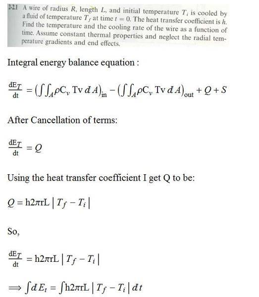
I'm really not sure, have I gone through the right process here?

I didn't actually finish the calculation, I'm just curious about the process.

 

[LawrenceC]

Pose the problem as a differential equation rather than integrals.

Equate the rate of heat loss due to convection from the radial surface to the rate of change of internal energy of the rod. This problem is considered a lumped mass situation. You should end up with a first order differential equation with temperature as the dependent variable and time as the independent variable.

 

[abstracted6]

Would you care to elaborate some more?

For your convenience, the photo at the bottom is from the main part of the section this problem is from:

 

[LawrenceC]

According to the problem, there is no thermal gradient in the radial (or any) direction. Therefore at any point in time, the temperature is uniform throughout the volume of the wire.

The heat loss is h*area*(T - Tinf). Units are energy per unit time

The heat loss equals the rate of change of energy in the wire. The energy in the wire is expressed as density*specific heat*volume*T. The unit is energy.

The rate of change of internal energy is

density*specific heat*volume*dT/dtheta, where theta is time. The units are energy per unit time.

Equate them and solve the ODE.

 

[LawrenceC]

In Equation 2.2-8, the only terms that apply here are dE/dt and Q. The rest are zero. There is no mass entering or leaving the control volume, and there is no heat generation.

 

[abstracted6]

I think I got it now, It didn't occur to me to actually write out the thermal energy in the control volume.

$$\frac{dE_T}{dt}=\frac{∂}{∂t}\int\int\int_\Omega \rho C_vTd\Omega$$
$$\frac{∂}{∂t}\int\int\int_\Omega \rho C_vTd\Omega=(\int\int_A \rho C_vTvdA)_{in}-(\int\int_A \rho C_vTvdA)_{out}+Q+S$$

From cancellation, simplification of terms:
$$\rho C_v\Omega\frac{dT}{dt}=Q$$
Also,
$$Q=h2\pi rL(T_i-T_f)$$

Combination/expansion of last two eqn's.
$$\rho C_v\pi r^2L\frac{dT}{dt}=h2\pi rL(T_i-T_f)$$

Simplify, solve for dT/dt
$$\frac{dT}{dt}=\frac{2h}{\rho C_vr}(T_i-T_f)$$

$$\implies\int dT=\frac{2h}{\rho C_vr}(T_i-T_f)\int dt$$

$$\implies T=\frac{2h}{\rho C_vr}(T_i-T_f)t+c_1$$

Initial condition, T(0)=T_i
$$T_i=0+c_1\implies c_1=T_i$$

So,
$$T(t)=\frac{2h}{\rho C_vr}(T_i-T_f)t+T_i$$
And,
$$\frac{d}{dt}T(t)=\frac{2h}{\rho C_vr}(T_i-T_f)$$

Look right?

 

[Chestermiller]

No. Q = 2πRL h (T_f - T ), not 2πRL h (T_f - T_i )

 

[LawrenceC]

Whenever you solve an engineering-type problem, look at your result to see if it makes sense with what you perceive to be reality. You have determined the temperature as a function of time. According to your result, the temperature change over any time interval is the same because your function is linear in time. Think of a cup of hot coffee at 200 F. In 20 seconds it will have cooled somewhat. Its mean temperature will have dropped x degrees. Now think about the coffee over the time interval of 5 minutes and 5 minutes plus 20 seconds. Would you expect the temperature drop to be the same? Suppose you go 10 minutes and 10 minutes plus 20 seconds. Would you again expect the temperature drop over that interval to be the same?

The linearity of your function indicates such would be the case. But we all know it isn't. The boundary condition is what drives this problem. Its strength depends on the difference between the object's temperature and the ambient temperature (and also some constants). Therefore its strength lessens in time because the temperature difference vanishes. Your result should reflect this.

 

[Chestermiller]

Whenever you solve an engineering-type problem, look at your result to see if it makes sense with what you perceive to be reality. You have determined the temperature as a function of time. According to your result, the temperature change over any time interval is the same because your function is linear in time. Think of a cup of hot coffee at 200 F. In 20 seconds it will have cooled somewhat. Its mean temperature will have dropped x degrees. Now think about the coffee over the time interval of 5 minutes and 5 minutes plus 20 seconds. Would you expect the temperature drop to be the same? Suppose you go 10 minutes and 10 minutes plus 20 seconds. Would you again expect the temperature drop over that interval to be the same?

The linearity of your function indicates such would be the case. But we all know it isn't. The boundary condition is what drives this problem. Its strength depends on the difference between the object's temperature and the ambient temperature (and also some constants). Therefore its strength lessens in time because the temperature difference vanishes. Your result should reflect this.

This is what I was trying to convey quantitatively in my post #7. The OP used an incorrect expression for calculating the heat flow rate. The heat flow rate is determined by the instantaneous temperature driving force between the cooling fluid and the wire.

 

[abstracted6]

So I will return to this step:

$$\frac{dT}{dt}=\frac{2h}{\rho C_vr}(T_i-T_f)$$

Which was supposed to be:

$$\frac{dT}{dt}=\frac{2h}{\rho C_vr}(T_f-T)$$

Since the last T now depends on time, I will need to move it over to the left of the equation.

$$\frac{dT}{dt}+\frac{2h}{\rho C_vr}T=\frac{2h}{\rho C_Vr}T_f$$

To make this easier to type I'm going to let,
$$n=\frac{2h}{\rho C_vr}$$
So,
$$T'(t)+nT(t)=nT_f$$

Use an integrating factor:
$$\mu T'(t)+\mu nT(t)=\mu nT_f$$

By inspection,
$$\frac{d}{dt}(T(t)e^{nt})=e^{nt}nT_f$$

$$T(t)e^{nt}=e^{nt}T_f+c_1$$
$$T(t)=T_f+e^{-nt}{c_1}$$

Initial condition: T(0)=T_i
$$T_i=T_f+c_1$$$$\implies c_1=T_i-T_f$$

So,
$$T(t)=T_f+e^{-\frac{2h}{\rho C_vr}t}(T_i-T_f)$$

Which looks like it makes since, as the temperature now varies as the inverse of the exponential function. Also as t goes to infinity, T(t) goes to T_f. And T(0) is T_i

 

[LawrenceC]

That's it.