Help with contour plots of effective potential in R3BP.

Join the discussion
Registration is free. Start your own thread to ask a follow-up.
1 reply · 3K views
Hjortlund
Messages
1
Reaction score
0
Hello everyone! I'm currently trying to plot the effective potential for Sun-Jupiter system, to show the lagrangian points in this system. I've converted to a system of units where G=1, m_sun+m_jupiter=1 and R=1, whereby I get the following equation describing the effective potential of a third mass m in the system:

U(x,y)=-1 * 0.999047/abs(sqrt((x-(-0.000953))^2 +y^2 ))-1 * 0.000953/abs(sqrt((x-0.999047)^2 +y^2 ))

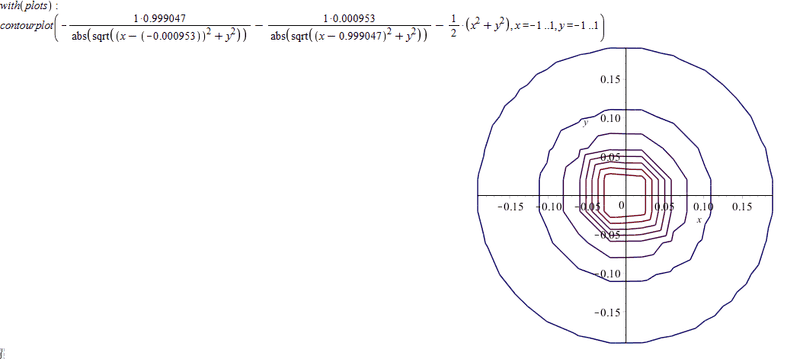
However, when I plot this in Maple, I don't get a contour plot that matches up with what I would expect
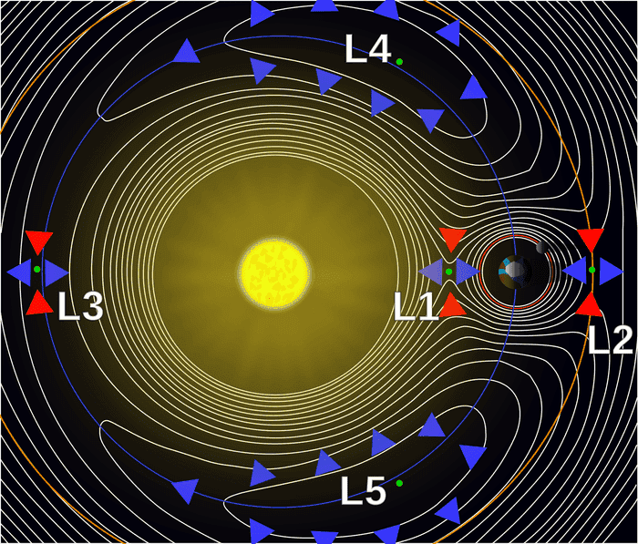
2000px-Lagrange_points2.svg.png

, but this.
oZLE3gV.png

Is there possibly anyone here who could point out a mistake I've done, or give me some advice? Thanks in advance!
 
Physics news on Phys.org
Welcome to PF!

I believe you are plotting the correct expression. But because the mass of Jupiter is much smaller than the mass of the sun, the Lagrange points are difficult to see on a contour plot. The Wikipedia site https://en.wikipedia.org/wiki/Lagrangian_point has some formulas for estimating where the points are located when one mass is much smaller than the other.

I tried a contour plot of your expression on Mathematica and I had to do quite a bit of playing around with the plotting parameters to see the contours near the Lagrange points. In particular, I had to zoom in on L3 and L4 and plot just a small region around the Lagrange points. I have not been able to get one plot that shows all the Lagrange points. Don't expect to get a plot that looks like the figure that you posted from the web site.

[EDIT: If you can "hand pick"" the value of each contour line, then you can get a pretty decent plot that shows all of the Lagrange points. Each contour line needs to be plotted with a sufficiently large number of points to get fairly smooth looking lines.]
 
Last edited: