MarkTheQuark
- 5
- 2
- TL;DR
- I need help plotting a parameter plane of energy-ratio R and the frequency-ratio of a spring pendulum.
I'm reading an article about the order-chaos-order sequence of a spring pendulum [Ref 1], as I'm reading it I'm trying to reproduce the graphs and results through Mathematica.
However, I am new to this software.
I will list below some of the most important equations mentioned in the paper.
"In its equilibrium position the spring will be stretched, due to the weight rng, to a length: ## l_c = l_0 + \frac{mg}{k} ##
angular frequency of the spring: ## \omega_s = \sqrt{\frac{k}{m}} ##
frequency of the pendulum: ## \omega_p = \sqrt{\frac{g}{l_c}} = \sqrt{\frac{g}{l_0 + mg/k}} ##
Total Energy: ## E = \frac{1}{2} m (\dot{x}^2 + \dot{y}^2) + mgy + \frac{1}{2} k (\sqrt{x^2 + y^2} - l_0)^2 ##
Minimum energy: ## E_{min} = -mg (l_0 + \frac{1}{2} \frac{mg}{k}) ##
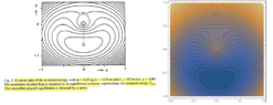
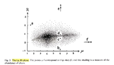
With that, the author makes a contour plot of the potential energy [Fig 1], and a Parameter Plane of R and ## \mu ## [Fig 2], where R and ## \mu ## are given by:
## R \equiv - \frac{E}{E_{min}} ##
## \mu = 1 + \frac{k l_0}{mg} ##
So, how did he found this parameter plane? And how can I remake it in Mathematica?
The article in question:
Ref 1 - The order—chaos—order sequence in the spring pendulum
J.P. van der Weele and E. de Kleine
Physica A: Statistical Mechanics and its Applications, 1996, vol. 228, issue 1, 245-272
Figures:
However, I am new to this software.
I will list below some of the most important equations mentioned in the paper.
"In its equilibrium position the spring will be stretched, due to the weight rng, to a length: ## l_c = l_0 + \frac{mg}{k} ##
angular frequency of the spring: ## \omega_s = \sqrt{\frac{k}{m}} ##
frequency of the pendulum: ## \omega_p = \sqrt{\frac{g}{l_c}} = \sqrt{\frac{g}{l_0 + mg/k}} ##
Total Energy: ## E = \frac{1}{2} m (\dot{x}^2 + \dot{y}^2) + mgy + \frac{1}{2} k (\sqrt{x^2 + y^2} - l_0)^2 ##
Minimum energy: ## E_{min} = -mg (l_0 + \frac{1}{2} \frac{mg}{k}) ##
With that, the author makes a contour plot of the potential energy [Fig 1], and a Parameter Plane of R and ## \mu ## [Fig 2], where R and ## \mu ## are given by:
## R \equiv - \frac{E}{E_{min}} ##
## \mu = 1 + \frac{k l_0}{mg} ##
So, how did he found this parameter plane? And how can I remake it in Mathematica?
The article in question:
Ref 1 - The order—chaos—order sequence in the spring pendulum
J.P. van der Weele and E. de Kleine
Physica A: Statistical Mechanics and its Applications, 1996, vol. 228, issue 1, 245-272
Figures: