How to plot integration equation using Python?

[Nur Ziadah]

I have a few of integration equations and need to convert it into Python. The problem is when I tried to plot a graph according to the equation, some of the plot is not same with the original one.

The first equation is the error probability of authentication in normal operation:

cond equation is the error probability of authentication under MIM attack:

The error probability of authentication in normal operation can be calculated by:

Supposedly, the graph (original) will be shown like this:

y-axis: error probability
x-axis: N
Pe^normal = blue lines
Pe^MIM = red lines
Differences between two error probabilities (Pe^MIM - Pe^normal)= green lines

I tried to code it into Python and this is my full codes:

import matplotlib.pyplot as plt
import math
import numpy as np
from scipy.special import iv,modstruve

x=np.arange(-0.5,21,1)
x = np.array(x)
t = 0.9
pe_normal = (np.exp(t*x/2)*(iv(0, t*x/2) - modstruve(0,t*x/2))-1)/(np.exp(t*x)-1)
pe_diff = (np.exp((1-t**2)*x/2)*(iv(0, (1-t**2)*x/2) - modstruve(0,(1-t**2)*x/2))-1)/(np.exp((1-t**2)*x)-1)
pe_mim= np.add(pe_normal,pe_diff)plt.plot(x, pe_normal, '-', color='blue', label='Normal')
plt.plot(x, pe_mim,  '-', color='red', label='MIM')
plt.plot(x, pe_diff,  '-', color='green', label='DIFF')
plt.xlabel('Mean photon number N')
plt.ylabel('Error probabiity')
plt.text(10, 0.4, 't=0.9', size=12, ha='center', va='center')
plt.ylim([0, 0.5])
plt.xlim([0, 20])
plt.legend()
plt.show()

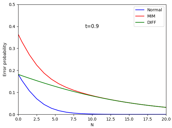
The graph produce from my code is:

It looks like that my plot is not same with the original one in terms N=0 of Pe^MIM (red line) and differences between two error probabilities (green line). The problem is the calculation for error probability under MIM attack was not given.

I hope that anyone may help me to solve this problem.

Thank you.

 

[jedishrfu]

Didn’t we discuss this program in this thread?

https://www.physicsforums.com/threads/convert-an-equation-to-python.962616/

Where you never responded to say whether it helped or not or have you fixed the expression I mentioned in it?

 

[Nur Ziadah]

Didn’t we discuss this program in this thread?

https://www.physicsforums.com/threads/convert-an-equation-to-python.962616/

Where you never responded to say whether it helped or not or have you fixed the expression I mentioned in it?

Thank you so much for your help. Apologize for not replying the threads. This post is different from the previous one.

 

[jedishrfu]

Ahh okay. I’ll look at it some more. Python and it’s plot capability is really awesome.

 

[Nur Ziadah]

Yes

Ahh okay. I’ll look at it some more. Python and it’s plot capability is really awesome.

Yes. It is very interesting to play around with python. However, I felt some headache to understand the equation.
Thank you for your attention and help for the previous post.
Really appreciate it.

 

[jedishrfu]

A couple of questions:

- so the t**2 means to square the t value right? Okay I found this is correct.

- and the z2 = y + z adds the elements of y to the elements of z to get an array of z2 right?

I thought maybe you need to use numpy to do the element by element addition.

I didn’t see the equation that you used to code the z = line

 

[jedishrfu]

For numpy:

z2 = np.add(y,z)

 

[Nur Ziadah]

A couple of questions:

- so the t**2 means to square the t value right? Okay I found this is correct.

- and the z2 = y + z adds the elements of y to the elements of z to get an array of z2 right?

I thought maybe you need to use numpy to do the element by element addition.

I didn’t see the equation that you used to code the z = line

1. Yes. t**2 is the square the t value
2. Yes. z2 = element of y + element of z
3. z line is (1-t**2)N, which is replacing tN in Pe^(aut,normal)

 

[Nur Ziadah]

For numpy:

z2 = np.add(y,z)

I have tried it. However, it shows the same graph that I have been plotted before.

 

[jedishrfu]

While I don’t see exactly what’s wrong, I do see places where you could improve the readability of your code.

1) use the same colors for the curves to make easier to compare the expected graph to the one you generated

2) label your variables like pe_mim, pe_normal, pe_diff

3) I don’t see where you’re doing the pe_diff calculation and this may be the source of your problem,

 

[Nur Ziadah]

For numpy:

z2 = np.add(y,z)

I have tried it. However, it shows the same graph that I have been plotted before.
View attachment 236522

While I don’t see exactly what’s wrong, I do see places where you could improve the readability of your code.

1) use the same colors for the curves to make easier to compare the expected graph to the one you generated

2) label your variables like pe_mim, pe_normal, pe_diff

3) I don’t see where you’re doing the pe_diff calculation and this may be the source of your problem,

I already updated the code and the graph in the question.

 

[Ibix]

Your curve for $P_e^{Auth,Normal}(t,N)$ looks right. Therefore the problem is in your MIM case. You don't seem to have written out an explicit expression for $P^{Auth,MIM}_e(t,N)$. Reverse engineering your code, you have implemented $$P_e^{Auth,MIM}(t,N)=
{{\left(I_0\left({{\left(1-t^2\right)N}\over{2}}\right)-
L_0\left({{\left(1-t^2\right)N}\over{2}}\right)
\right)e^{{{\left(1-t^2\right)N}/{2}}}-1}\over{e^{\left(1-t^
2\right)N}-1}}+{{\left(I_0\left({{tN}\over{2}}\right)-
L_0\left({{tN}\over{2}}\right)\right)e^{{{tN
}/{2}}}-1}\over{e^{tN}-1}}$$(Edit: replaced x with N above.) I presume this is incorrect.

 

[Nur Ziadah]

Your curve for $P_e^{Auth,Normal}(t,N)$ looks right. Therefore the problem is in your MIM case. You don't seem to have written out an explicit expression for $P^{Auth,MIM}_e(t,N)$. Reverse engineering your code, it is $$P_e^{Auth,MIM}(t,N)=
{{\left(I_0\left({{\left(1-t^2\right)x}\over{2}}\right)-
L_0\left({{\left(1-t^2\right)x}\over{2}}\right)
\right)e^{{{\left(1-t^2\right)x}/{2}}}-1}\over{e^{\left(1-t^
2\right)x}-1}}-{{\left(I_0\left({{tx}\over{2}}\right)-
L_0\left({{tx}\over{2}}\right)\right)e^{{{tx
}/{2}}}-1}\over{e^{tx}-1}}$$I presume this is incorrect.

How to write the expression for $P^{Auth,MIM}_e(t,N)$? Do you have any idea, what is the equation to plot $P^{Auth,MIM}_e(t,N)$?

 

[Ibix]

I've no idea. I simply reverse engineered your code in the hope that you would see a typo or something.

You seem to have a source with at least some of the maths in it - what does it say? And you have the graph you want to replicate - how was it generated?

 

[Ibix]

I simply reverse engineered your code in the hope that you would see a typo or something.

...speaking of which, it should be a plus between the fractions. Now corrected above.

 

[Nur Ziadah]

...speaking of which, it should be a plus between the fractions. Now corrected above.

Yes. I realized it. It is stated that

. However, I don't think that they used another equation to calculate pe_mim.

 

[Ibix]

Then what is the expression given for the difference? Is it consistent with the expression I gave in #12?

 

[Nur Ziadah]

Actually, I didn't have any idea.

 

[Ibix]

Then where did you get what you implemented in the code?

 

[Nur Ziadah]

Then where did you get what you implemented in the code?

I will try to ask about the equation from the author of the paper. Hopefully he will response my questions.

 

[Ibix]

A good idea. It seems to me that the problem is you don't know what to plot, not a problem with the actual plotting. You might get more help with that if you provide a link to the paper and start a thread asking for help understanding that, rather than focussing on the python. Your code seems to be right in the sense that it's doing what you ask - your problem is that you don't know what exactly you want it to do.

 

[Nur Ziadah]

A good idea. It seems to me that the problem is you don't know what to plot, not a problem with the actual plotting. You might get more help with that if you provide a link to the paper and start a thread asking for help understanding that, rather than focussing on the python. Your code seems to be right in the sense that it's doing what you ask - your problem is that you don't know what exactly you want it to do.

That is the good idea. I will start a new thread and asking about the equations.