How to solve Diffusion Equation with time dependant conditions?

[Zimbalj]

TL;DR Summary

By which method could i analytically solve Diffusion Equation with this boundary conditions:

U=U(x,t)

Ut=DUxx; 0<=x<=L, t>0

U(x,0)=0 0<x<=L
U(0,t)=a(t); t>0 *a(t) is known function*
(dU/dx)=0 for x=L

I have looked into many ways but not one is usable for diffusion equation with this boundary conditions.

 

[fresh_42]

How far did you come?

You should also check the last attachment in
https://www.physicsforums.com/threads/solution-manuals-for-the-math-challenges.977057/
(problem 14 Nov. 2020)

 

[Zimbalj]

Standard method of separation by variables does not match up nicely with boundary conditions. I have seen methods for solving inhomogeneous heat equation using green functions, but that again failed, because it required knowledge of U(L,t) which was not given by any condition

 

[Zimbalj]

How far did you come?

You should also check the last attachment in
https://www.physicsforums.com/threads/solution-manuals-for-the-math-challenges.977057/
(problem 14 Nov. 2020)

November 2020 does have diffusion equation problem, but i do not know how to use any of information there to solve my problem. Soluton on picturem from the book is the case that mostly resembles my problem, but again i need boundary condition U(L,t)=b(t), instead i have flux that equals zero at that point U'(L,t)=0, so i can't use that metod

 

[bigfooted]

The idea behind solving the source-on-the-half-line problem is to transform the PDE for U with nonhomogeneous boundary conditions into another PDE for V with homogeneous boundary conditions, as is done in the attachment that you've posted.

 

[Paul Colby]

I don’t see why separation of variables isn’t a good start? For a separation constant, $\omega$, the solution with $u’_\omega(t,L)=0$ is,

$u_\omega(t,x) = e^{\omega t}\cosh(\sqrt{\omega}(x-L))$

So, the solution you seek is some weighted sum over $\omega$. Evaluating at $x=0$ gives,

$u_\omega(t,0)=\cosh(\sqrt{\omega}L)e^{\omega t}$

this will lead to an answer in terms of Laplace transforms.

 

[Zimbalj]

The problem is boundary condition that is time dependant:
U(0,t)=a(t)
With constant boundary condition i get analytical solution relatively easy, but with time dependant boundary condition i always get that some of the integration constants are functions of t which is not right

Lets say:
U(x,t)=A(x)B(t)

U(0,t)=A(0)B(t)=a(t) => B(t)=a(t)/A(0) *A(0) should be some constant

but function a(t) is not in a form that resembles solution for the time part, when the equation is separated

B_t+(Dw²)B=0

 

[fresh_42]

The problem is boundary condition that is time dependant:
U(0,t)=a(t)
With constant boundary condition i get analytical solution relatively easy, but with time dependant boundary condition i always get that some of the integration constants are functions of t which is not right

Lets say:
U(x,t)=A(x)B(t)

U(0,t)=A(0)B(t)=a(t) => B(t)=a(t)/A(0) *A(0) should be some constant

but function a(t) is not in a form that resembles solution for the time part, when the equation is separated

B_t+(Dw²)B=0

Have a look at 16.1. in
https://web.math.ucsb.edu/~grigoryan/124A/lecs/lec16.pdf
And
https://web.math.ucsb.edu/~grigoryan/124A/lecs/
is the list of all lectures of the course.

 

[Zimbalj]

Have a look at 16.1. in
https://web.math.ucsb.edu/~grigoryan/124A/lecs/lec16.pdf
And
https://web.math.ucsb.edu/~grigoryan/124A/lecs/
is the list of all lectures of the course.

Thanks, i will. Although at 16.1 they give solution to wave equation, i think i may use this method for my diffusion equation, i will try.

 

[Paul Colby]

With constant boundary condition i get analytical solution relatively easy, but with time dependant boundary condition i always get that some of the integration constants are functions of t which is not right

That is what the Laplace transform is all about. To find the weight in the weighted sum, one must take an inverse Laplace transform. One must also meet the $t=0$ boundary value by selecting appropriate constants.

 

[Zimbalj]

Thanks. I tried Laplace transform L[U(x,t)]=V(x,s) and got:

Vxx-s/D*V=0

sorry for my bad writing of formulas, i am new at LaTeX.

With problematic boundary condition getting form

V(0,s)=A(s)

 

[Paul Colby]

sorry for my bad writing of formulas, i am new at LaTeX.

You should follow some of the how to docs for this forum.

I tried Laplace transform L[U(x,t)]=V(x,s) and got:

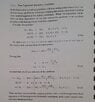
What you tried isn’t what I’m suggesting. I’ve provided explicit solutions to the heat equation that all obey the boundary condition, $u’(t,L)=0$, for all $t$. With a slight and obvious modification, we can make these solutions also all obey the boundary condition, $u(0,x)=0$, for all $x$. These solution are just linear combinations of the original set,

$u_\omega(t,x)= \cosh(\sqrt{\omega}(x-L)(e^{\omega t}-1)$[1]

notice that $u_\omega(0,x)=0$. So, I’ve provided a set of solutions to the heat equation indexed by a complex parameter, $\omega$, all of which obey 2 out of the three boundary conditions. The final boundary condition, $u(t,0)=a(t)$, may be expressed as an integral equation of the first kind,

$a(t)=\int A(\omega)u_\omega(t,0)d\omega$, (*)

making the solution to the stated problem,

$u(t,x)=\int A(\omega)u_\omega(t,x)d\omega$

Relating Equation (*) to an inverse Laplace transform is left to the reader.

[1] yeah, I see the problem the problem here. $\cosh(x)$ isn’t a solution. Oh well.

 

[Paul Colby]

Even with its flaws the approach in the previous post still has promise, which is why I’ll leave it as is. it is still possible to take,

$u_\omega(t,x)=\cosh(\sqrt{\omega}(x-L))e^{\omega t}$

as the kernel in the previous post. One just has to add the additional condition,

$0 = \int A(\omega)u_\omega(0,x)d\omega$

 

[Zimbalj]

The equation is left unsolved, but that is not a big deal. Thanks everyone for insights, it will be helpful in future, because I will try to solve some other similar equations.