mathmari
Gold Member
MHB
- 4,984
- 7
Hey! 
I want to determine an approximation of a cubic polynomial that has at the points $$x_0=-2, \ x_1=-1, \ x_2=0 , \ x_3=3, \ x_4=3.5$$ the values $$y_0=-33, \ y_1=-20, \ y_2=-20.1, \ y_3=-4.3 , \ y_4=32.5$$ using the least squares method.
So we are looking for a cubic polynomial $p(x)$ such that $$\sum_{i=0}^4\left (p(x_i)-y_i\right )^2$$ is minimal, right? (Wondering) Let $p(x)=a_3x^3+a_2x^2+a_1x+a_0$. Then we get the following sum:
\begin{align*}\sum_{i=0}^4\left (p(x_i)-y_i\right )^2=&\left (-8a_3+4a_2-2a_1+a_0+33\right )^2+\left (-a_3+a_2-a_1+a_0+20\right )^2+\left (a_0+20.1\right )^2 \\ & +\left (27a_3+9a_2+3a_1+a_0+4.3\right )^2 +\left (42.875a_3+12.25a_2+3.5a_1+a_0-32.5\right )^2\end{align*}
Now we calculate the partial derivatives in respect to each $a_i$ and then we set these equal to $0$. In that we get a system of equations.
Let this sum be $S$.
We get the following partial derivatives:
\begin{align*}\frac{\partial{S}}{\partial{a_0}}=&2\left (-8a_3+4a_2-2a_1+a_0+33\right )+2\left (-a_3+a_2-a_1+a_0+20\right )\\ & +2\left (a_0+20.1\right ) +2\left (27a_3+9a_2+3a_1+a_0+4.3\right ) +2\left (42.875a_3+12.25a_2+3.5a_1+a_0-32.5\right )\\ = &89.8 + 10 a_0 + 7 a_1+ 52.5 a_2 + 121.75 a_3\end{align*}
\begin{align*}\frac{\partial{S}}{\partial{a_1}}=&2\left (-8a_3+4a_2-2a_1+a_0+33\right )\cdot 2+2\left (-a_3+a_2-a_1+a_0+20\right )\cdot (-1) \\ & +2\left (27a_3+9a_2+3a_1+a_0+4.3\right )\cdot 3 +2\left (42.875a_3+12.25a_2+3.5a_1+a_0-32.5\right )\cdot 3.5 \\ = & -109.7 + 15 a_0 + 36.5 a_1 + 153.75 a_2 + 432.125 a_3\end{align*}
\begin{align*}\frac{\partial{S}}{\partial{a_2}}=&2\left (-8a_3+4a_2-2a_1+a_0+33\right )\cdot 4+2\left (-a_3+a_2-a_1+a_0+20\right ) \\ & +2\left (27a_3+9a_2+3a_1+a_0+4.3\right )\cdot 9 +2\left (42.875a_3+12.25a_2+3.5a_1+a_0-32.5\right )\cdot 12.25\\ = & -414.85 + 52.5 a_0 + 121.75 a_1 + 496.125 a_2 + 1470.44 a_3 \end{align*}
\begin{align*}\frac{\partial{S}}{\partial{a_3}}=&2\left (-8a_3+4a_2-2a_1+a_0+33\right )\cdot (-8)+2\left (-a_3+a_2-a_1+a_0+20\right )\cdot (-1) \\ & +2\left (27a_3+9a_2+3a_1+a_0+4.3\right )\cdot 27 +2\left (42.875a_3+12.25a_2+3.5a_1+a_0-32.5\right )\cdot 42.875\\ = & -3122.68 + 121.75 a_0 + 496.125 a_1 + 1470.44 a_2 + 5264.53 a_3\end{align*}
So, we get the system:
\begin{align*}& \ \ \ \ 89.8 + 10 a_0 + 7 a_1+ 52.5 a_2 + 121.75 a_3=0 \\ &-109.7 + 15 a_0 + 36.5 a_1 + 153.75 a_2 + 432.125 a_3=0 \\ &-414.85 + 52.5 a_0 + 121.75 a_1 + 496.125 a_2 + 1470.44 a_3=0 \\ &-3122.68 + 121.75 a_0 + 496.125 a_1 + 1470.44 a_2 + 5264.53 a_3=0\end{align*}
Then we get the solution: \begin{equation*}a_0\approx -21.6611, \ a_1\approx -7.08875, \ a_2\approx -2.0.6057, \ a_3\approx 2.33768\end{equation*}
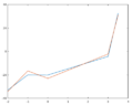
The cubic polynomial that we are looking for is \begin{equation*}p(x)=2.33768x^3-2.0.6057x^2-7.08875x-21.6611 \end{equation*}
Doing the above in an other way I got an other result, but I don't know why and which is the correct one. (Wondering)
Using the least square method and the normal equation we get that the solution that we are looking for is the vector $\vec{a}$ such that $A \vec{a}=b \Rightarrow A^TA\vec{a}=A^Tb$.
So we get the following:
\begin{equation*}
\begin{bmatrix}
5 & 3.5 & 26.25 & 60.875 \\
3.5 & 26.25 & 60.875 & 248.0625 \\
26.25 & 60.875 & 248.0625 & 735.21875 \\
60.875 & 248.0625 & 735.21875 & 2632.265625
\end{bmatrix}
\begin{bmatrix}
a_0 \\
a_1 \\
a_2 \\
a_3 \\
\end{bmatrix}=
\begin{bmatrix}
-44.9 \\
186 \\
207.425 \\
1561.3375 \\
\end{bmatrix}
\end{equation*}
Solving this one we get the polynomial $$p(x)=-23.0087-12.2424x-2.7837x^2+3.0565x^3$$ This is not the same polynomial as the one that we get at the first method. And for the second polynomial the condition $p(0)=-20.1$ is not true. (Wondering)
I want to determine an approximation of a cubic polynomial that has at the points $$x_0=-2, \ x_1=-1, \ x_2=0 , \ x_3=3, \ x_4=3.5$$ the values $$y_0=-33, \ y_1=-20, \ y_2=-20.1, \ y_3=-4.3 , \ y_4=32.5$$ using the least squares method.
So we are looking for a cubic polynomial $p(x)$ such that $$\sum_{i=0}^4\left (p(x_i)-y_i\right )^2$$ is minimal, right? (Wondering) Let $p(x)=a_3x^3+a_2x^2+a_1x+a_0$. Then we get the following sum:
\begin{align*}\sum_{i=0}^4\left (p(x_i)-y_i\right )^2=&\left (-8a_3+4a_2-2a_1+a_0+33\right )^2+\left (-a_3+a_2-a_1+a_0+20\right )^2+\left (a_0+20.1\right )^2 \\ & +\left (27a_3+9a_2+3a_1+a_0+4.3\right )^2 +\left (42.875a_3+12.25a_2+3.5a_1+a_0-32.5\right )^2\end{align*}
Now we calculate the partial derivatives in respect to each $a_i$ and then we set these equal to $0$. In that we get a system of equations.
Let this sum be $S$.
We get the following partial derivatives:
\begin{align*}\frac{\partial{S}}{\partial{a_0}}=&2\left (-8a_3+4a_2-2a_1+a_0+33\right )+2\left (-a_3+a_2-a_1+a_0+20\right )\\ & +2\left (a_0+20.1\right ) +2\left (27a_3+9a_2+3a_1+a_0+4.3\right ) +2\left (42.875a_3+12.25a_2+3.5a_1+a_0-32.5\right )\\ = &89.8 + 10 a_0 + 7 a_1+ 52.5 a_2 + 121.75 a_3\end{align*}
\begin{align*}\frac{\partial{S}}{\partial{a_1}}=&2\left (-8a_3+4a_2-2a_1+a_0+33\right )\cdot 2+2\left (-a_3+a_2-a_1+a_0+20\right )\cdot (-1) \\ & +2\left (27a_3+9a_2+3a_1+a_0+4.3\right )\cdot 3 +2\left (42.875a_3+12.25a_2+3.5a_1+a_0-32.5\right )\cdot 3.5 \\ = & -109.7 + 15 a_0 + 36.5 a_1 + 153.75 a_2 + 432.125 a_3\end{align*}
\begin{align*}\frac{\partial{S}}{\partial{a_2}}=&2\left (-8a_3+4a_2-2a_1+a_0+33\right )\cdot 4+2\left (-a_3+a_2-a_1+a_0+20\right ) \\ & +2\left (27a_3+9a_2+3a_1+a_0+4.3\right )\cdot 9 +2\left (42.875a_3+12.25a_2+3.5a_1+a_0-32.5\right )\cdot 12.25\\ = & -414.85 + 52.5 a_0 + 121.75 a_1 + 496.125 a_2 + 1470.44 a_3 \end{align*}
\begin{align*}\frac{\partial{S}}{\partial{a_3}}=&2\left (-8a_3+4a_2-2a_1+a_0+33\right )\cdot (-8)+2\left (-a_3+a_2-a_1+a_0+20\right )\cdot (-1) \\ & +2\left (27a_3+9a_2+3a_1+a_0+4.3\right )\cdot 27 +2\left (42.875a_3+12.25a_2+3.5a_1+a_0-32.5\right )\cdot 42.875\\ = & -3122.68 + 121.75 a_0 + 496.125 a_1 + 1470.44 a_2 + 5264.53 a_3\end{align*}
So, we get the system:
\begin{align*}& \ \ \ \ 89.8 + 10 a_0 + 7 a_1+ 52.5 a_2 + 121.75 a_3=0 \\ &-109.7 + 15 a_0 + 36.5 a_1 + 153.75 a_2 + 432.125 a_3=0 \\ &-414.85 + 52.5 a_0 + 121.75 a_1 + 496.125 a_2 + 1470.44 a_3=0 \\ &-3122.68 + 121.75 a_0 + 496.125 a_1 + 1470.44 a_2 + 5264.53 a_3=0\end{align*}
Then we get the solution: \begin{equation*}a_0\approx -21.6611, \ a_1\approx -7.08875, \ a_2\approx -2.0.6057, \ a_3\approx 2.33768\end{equation*}
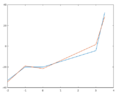
The cubic polynomial that we are looking for is \begin{equation*}p(x)=2.33768x^3-2.0.6057x^2-7.08875x-21.6611 \end{equation*}
Doing the above in an other way I got an other result, but I don't know why and which is the correct one. (Wondering)
Using the least square method and the normal equation we get that the solution that we are looking for is the vector $\vec{a}$ such that $A \vec{a}=b \Rightarrow A^TA\vec{a}=A^Tb$.
So we get the following:
\begin{equation*}
\begin{bmatrix}
5 & 3.5 & 26.25 & 60.875 \\
3.5 & 26.25 & 60.875 & 248.0625 \\
26.25 & 60.875 & 248.0625 & 735.21875 \\
60.875 & 248.0625 & 735.21875 & 2632.265625
\end{bmatrix}
\begin{bmatrix}
a_0 \\
a_1 \\
a_2 \\
a_3 \\
\end{bmatrix}=
\begin{bmatrix}
-44.9 \\
186 \\
207.425 \\
1561.3375 \\
\end{bmatrix}
\end{equation*}
Solving this one we get the polynomial $$p(x)=-23.0087-12.2424x-2.7837x^2+3.0565x^3$$ This is not the same polynomial as the one that we get at the first method. And for the second polynomial the condition $p(0)=-20.1$ is not true. (Wondering)