Question about computing diffraction patterns

[Ax_xiom]

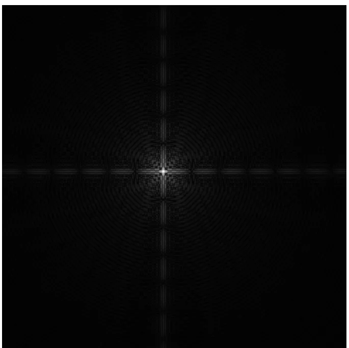
So I'm using python to compute the fourier transform of a black and white image and the images I've been getting have been different to what I expected.

Input image:

Output FFT:

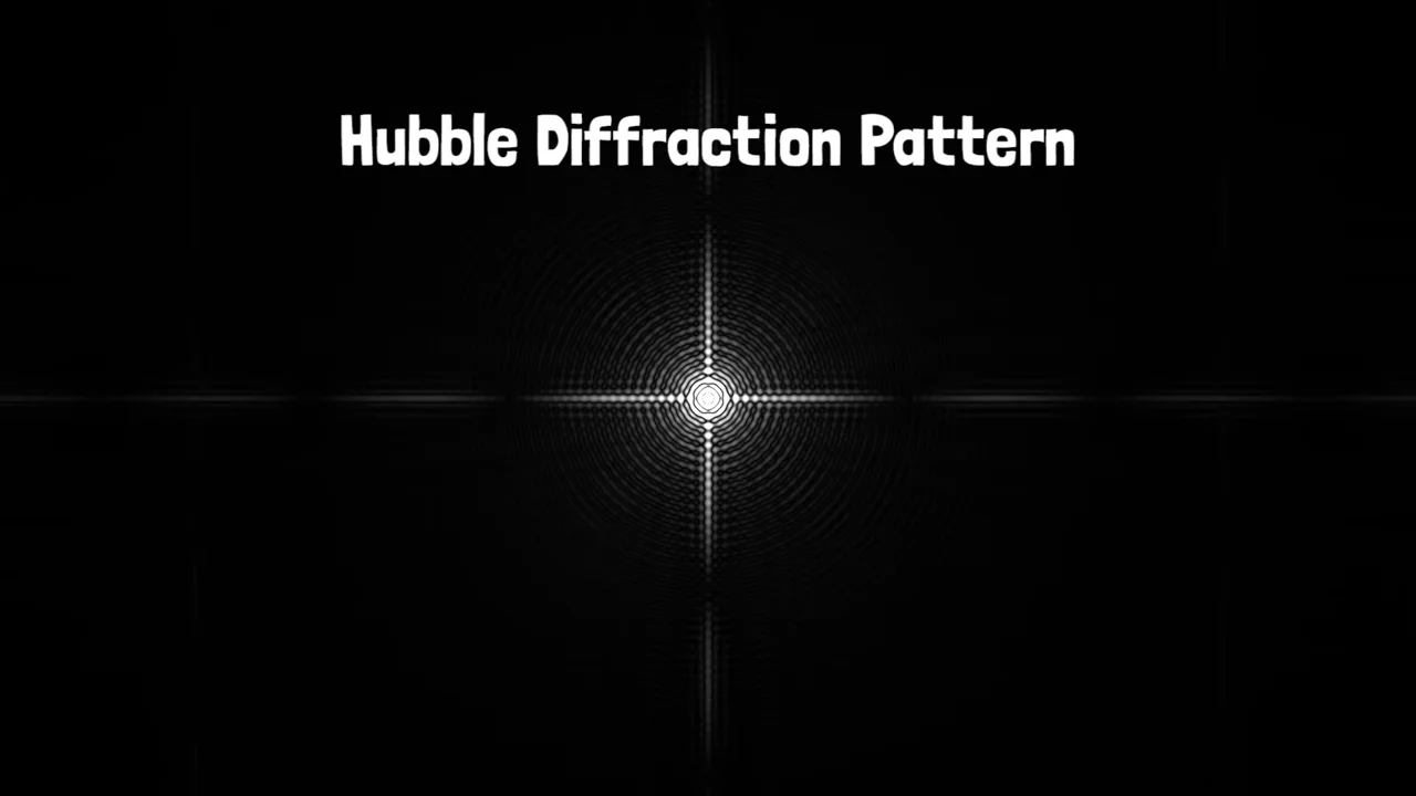
What I expected:

Image from MinutePhysics's video Why are Stars Star-Shaped?

So why is there a difference?

 

[Ibix]

The aperture of Hubble is round and the spider legs are connected to it. With the aperture function you've drawn you are not modelling the telescope tube at all, just the secondary and its legs floating in empty space. I suspect you have the spider legs too thick as well, although I haven't checked. Try something more like this:

Also remember that numeric computation does a discrete FFT, not a continuous one. Are you padding and block swapping your aperture function before the transform?

 

[Ax_xiom]

Try something more like this:

I tried it and I get this:

Which does have the same general structure as what I'm aiming for, but doesn't "glow" as much

Are you padding and block swapping your aperture function before the transform?

Here is the code I'm using, I'm not sure if it uses block swapping

 

[Ibix]

Blockswapping is what fftshift does. You want the center of the aperture at [0,0] before the FFT.

The page you linked is a generic page about doing FFTs. It would probably help if you posted your actual code. You can use code=python tags like this:

print("Hello world!")

 

[Ax_xiom]

Blockswapping is what fftshift does. You want the center of the aperture at [0,0] before the FFT.

I'll create a new image with the centre at 0,0 so no shifting is required.

The page you linked is a generic page about doing FFTs. It would probably help if you posted your actual code. You can use code=python tags like this:

Here it is:

# fourier_synthesis.py

import numpy as np
import matplotlib.pyplot as plt

image_filename = "HubbleOutline10.jpg"

def calculate_2dft(input):
    ft = np.fft.ifftshift(input)
    ft = np.fft.fft2(ft)
    return np.fft.fftshift(ft)

# Read and process image
image = plt.imread(image_filename)
image = image[:, :, :3].mean(axis=2)  # Convert to grayscale

plt.set_cmap("gray")

ft = calculate_2dft(image)

plt.subplot(121)
plt.imshow(image)
plt.axis("off")
plt.subplot(122)
plt.imshow(abs(ft)**0.5)
plt.axis("off")
plt.show()

 

[sbrothy]

I'll create a new image with the centre at 0,0 so no shifting is required.

Here it is:

# fourier_synthesis.py

import numpy as np
import matplotlib.pyplot as plt

image_filename = "HubbleOutline10.jpg"

def calculate_2dft(input):
    ft = np.fft.ifftshift(input)
    ft = np.fft.fft2(ft)
    return np.fft.fftshift(ft)

# Read and process image
image = plt.imread(image_filename)
image = image[:, :, :3].mean(axis=2)  # Convert to grayscale

plt.set_cmap("gray")

ft = calculate_2dft(image)

plt.subplot(121)
plt.imshow(image)
plt.axis("off")
plt.subplot(122)
plt.imshow(abs(ft)**0.5)
plt.axis("off")
plt.show()

Coming from C/C++ and DirectX (and now the outdated OpenGL), I'm always flabbergasted at the shortness of these "scripts".

 

[Ibix]

I'll create a new image with the centre at 0,0 so no shifting is required.

Here it is:

# fourier_synthesis.py

import numpy as np
import matplotlib.pyplot as plt

image_filename = "HubbleOutline10.jpg"

def calculate_2dft(input):
    ft = np.fft.ifftshift(input)
    ft = np.fft.fft2(ft)
    return np.fft.fftshift(ft)

# Read and process image
image = plt.imread(image_filename)
image = image[:, :, :3].mean(axis=2)  # Convert to grayscale

plt.set_cmap("gray")

ft = calculate_2dft(image)

plt.subplot(121)
plt.imshow(image)
plt.axis("off")
plt.subplot(122)
plt.imshow(abs(ft)**0.5)
plt.axis("off")
plt.show()

Looks sensible. Except why are you taking $\sqrt{|F|}$? Surely you just want the absolute value. Also , don't use jpg for binary images, because the compression causes ringing. Use something lossless - a bmp or a png or gif.

 

[Ax_xiom]

Looks sensible. Except why are you taking $\sqrt{|F|}$? Surely you just want the absolute value. Also , don't use jpg for binary images, because the compression causes ringing. Use something lossless - a bmp or a png or gif.

I'm taking the square root so the image looks brighter compare the regular image

to the image when the values are squarerooted

The squarerooted version is the closest to what I'm trying to do, but my target image has the centre much brighter and the edges much darker

 

[Ibix]

On the subject of brightness, the typical way of dealing with this would be np.log(1+abs(ft)). Also, look at the documentation for imshow. Does it scale the output so that the brightest point is 255? If not, do that.

Let's do some maths. Under discrete FT, the 1d top hat function ($f(x)=1$ for $|x|<W/2$, 0 otherwise) transforms to $$F(k)=\frac{\sin(\pi W k/N)}{\sin(\pi k/N)}$$(Wikipedia) where $N$ is the number of pixels across your image and $W$ is the top hat function width in pixels. Eyeballing your image, you have $W/N\approx 0.1$, so you would get this:

If you plug in $W/N=0.9$ you would get this:

The latter looks to me more like what you are expecting, so make your aperture much larger - play around with 50-90% of the width of your image. Up the number of pixels if you want more detail (FFTs work well with powers of two pixel sizes - I think FFTW underlies python's DFFT and that's more flexible, but $2^n\times 2^n$ is always good).

Note: the 1d transform I've shown is a cross-section of a square aperture, so won't exactly match a cross-section of the FT of a round aperture, which would be a Bessel function of the first kind. It's close enough for jazz. Your aperture function is also more complicated than a simple top hat, so you don't expect it to match anyway. That's why you'll need to play around with the scale to get something that looks similar to the original image.

 

[Ibix]

Just to note, the reason the size of the aperture in relation to the size of the image matters is that (given a fixed aperture size that you are actually modelling) this ratio defines your sample density in Fourier space. The continuous FT of the aperture is always the same, but by varying $W/N$ you vary the scale of the grid of points in Fourier space that you sample to form your output image.

In the actual telescope the physical size of the diffraction pattern depends on the optics - mainly on the size of the primary mirror, which is part of why bigger is better in telescopes (within limits). If you know enough about the optics you can work out the scale and then adjust the image and aperture size so the output sampling is the same as the CCD in the telescope. I suspect the sampling in the original image is probably finer than the actual instrument, though, because what that pattern tells you is how fine-grained a CCD it's worth buying. You can't see real detail below the scale of the diffraction pattern because that pattern is the "blur" induced by your optics, so it isn't worth buying a CCD finer than that because you'd be spending money to see the diffraction patterns better, not the stars.

Side note: the density of photoreceptors in the fovea closely matches that sampling limit for the optics of a human eye. Evolution in action again.