Time evolution of the electromagnetic wavefunction on a lattice

Join the discussion
Registration is free. Ask a follow-up in this thread, or start your own.
9 replies · 3K views · last reply
James1238765
Messages
120
Reaction score
8
TL;DR
Why does this time evolution of the electromagnetic wavefunction diverges?
The Maxwell wavefunction of a photon is given in [here] as follows:
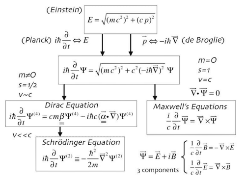
Flowchart of wave equations: Einstein's energy-momentum relation E = sqrt((mc^2)^2 + (cp)^2) leads via Planck and de Broglie substitutions to a general wave equation, which branches into the Dirac equation (m not 0, spin 1/2) and Maxwell's equations (m=0, spin 1, v=c).

Because the curl operation mixes 3 different components, this wavefunction only works for a minimum of 3 space dimensions, with each grid point having 6 component numbers ##{E^1, E^2, E^3, B^1, B^2, B^3}##, and with the following update rules:

$$ E_{x,y,z}^1 = E_{x,y,z}^1 + B_{x,y+1,z}^3 - B_{x,y,z}^3 - B_{x,y,z+1}^2 + B_{x,y,z}^2$$
$$ E_{x,y,z}^2 = E_{x,y,z}^2 + B_{x,y,z+1}^1 - B_{x,y,z}^1 - B_{x+1,y,z}^3 + B_{x,y,z}^3$$
$$ E_{x,y,z}^3 = E_{x,y,z}^3 + B_{x+1,y,z}^2 - B_{x,y,z}^2 - B_{x,y+1,z}^1 + B_{x,y,z}^1$$
$$ B_{x,y,z}^1 = B_{x,y,z}^1 - E_{x,y+1,z}^3 + E_{x,y,z}^3 + E_{x,y,z+1}^2 - E_{x,y,z}^2$$
$$ B_{x,y,z}^2 = B_{x,y,z}^2 - E_{x,y,z+1}^1 + E_{x,y,z}^1 + E_{x+1,y,z}^3 - E_{x,y,z}^3$$
$$ B_{x,y,z}^3 = B_{x,y,z}^3 - E_{x+1,y,z}^2 + E_{x,y,z}^2 + E_{x,y+1,z}^1 - E_{x,y,z}^1$$

corresponding to ##\frac{dE}{dt} = \nabla x B## and ##\frac{dB}{dt} = - \nabla x E##

The complicated time evolution due to the mixing of the 6 components over time gives rise to complex behavior, which are not intuitive to predict.

1.
Setting E1 = 1 over all ##[x,y,z]## points in the 3 dimensional grid, and setting all other components E2, E3, B1, B2, B3 = 0 all over the grid, we obtain:
Small yellow graphic with red text reading EX at [50,50,50], with a short red tick mark and a short pink tick mark on the left edge.


with no time evolution of any components throughout the grid.

2.
Setting E1 = ##sin (\frac{x}{width}2\pi) ## over all [x,y,z] points in the grid, and setting all other components to 0, we obtain:
Small yellow image with red text reading "EX at [50,50,50]" and a short red tick mark and a faint pink tick mark along the left edge.


still without time evolution.

3.
Setting Ei = ##sin (\frac{i}{width}2\pi) ## for all the 6 components:
Yellow rectangle with red text reading E1, E2, E3, B1, B2, B3 at [50,50,50].


still produces no time evolution! The curl operation is rather finicky.

4.
Setting E1 = ##sin (\frac{x+y+z}{width}2\pi) ## and ## E2, E3, E4, E5, E6 = 0 ## everywhere:
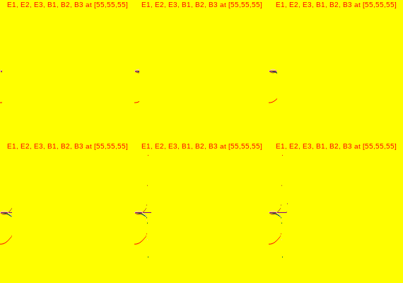
Small yellow image with red text reading E1, E2, E3, B1, B2, B3 at [55,55,55], plus a few tiny stray marks along the left edge.


finally produces a time evolution.

However the time evolution explodes partway, as shown in the chart, and the numerical data below.
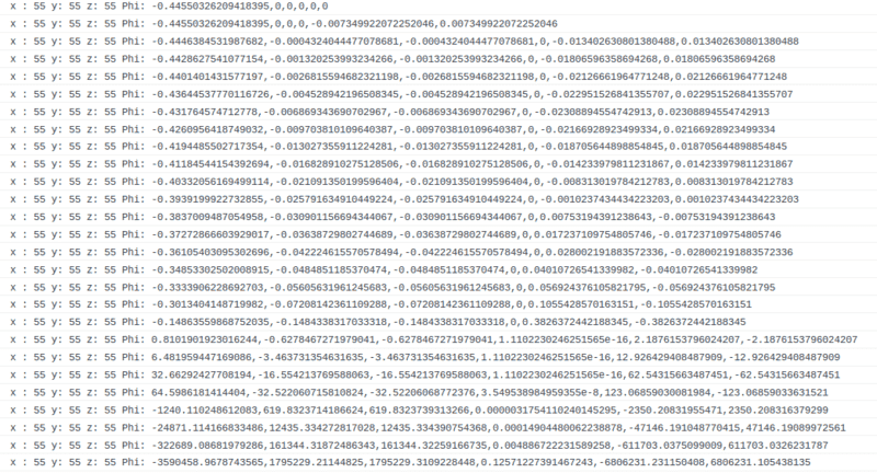
Plain-text table of numeric output rows labelled x, y, z and Phi1, with values such as -0.4455 and 0.0073 that vary across successive lines.


I am unsure why this happens, because the update rules involve only additions (with no multiplications or other fancy operations)?
 
Last edited:
Physics news on Phys.org
I have my doubts about the maxwell wavefunction of the photon idea, but for Maxwell’s equations just from poking around the web, people seem to use FDTD (also called Yee’s method) for the discretization which staggers E and H in time and space.
 
  • Like
Likes   Reactions: James1238765
@Frabjous thank you. i am interested in these multi-dimensional cross relationships between lattice grid components over time. In the 8-components Dirac equation, a similar looking complicated time evolution relationship also exists between the individual components.

Is there a name for the mathematical branch that can analyze the behavior over time of these kind of self interacting components?
 
Sorry, I have not been exposed to that. My generic advice is that these are really ugly equations to solve in general. You need to get specific about the problem you are trying to solve and then try to find a technique. As you discovered above, stability conditions can kill you.
 
I would call this finite element analysis. FYI.... Folks usually don't start by solving eight component fields in four+ dimensions. Perhaps a more measured approach would serve you better?
 
@hutchphd I am familiar with the discretization and computation aspects using finite elements. Can finite elements methods also analyze for instance which initial conditions with be stable over time and which will not, *without doing the computation*? Can you link to which method in finite elements allows us to do this?
 
No I cannot. These are not easy and only rarely yield to clever analytic manipulation Nobel prizes have been sometimes involved.
 
@hutchphd thank you. You seem to hint towards the Navier Stokes wave, so while at it I translated the usual equations into the same notation as above for future reference. There are 3 velocity component numbers ##\{u, v, w\}## in the 3 dimensional Navier Stokes grid ##[x, y, z]##:

$$ \frac{du}{dt} = \frac{d^2u}{dx^2} + \frac{d^2u}{dy^2} + \frac{d^2u}{dz^2} - u\frac{du}{dx} - v\frac{du}{dy} - w\frac{du}{dz}$$
$$ \frac{dv}{dt} = \frac{d^2v}{dx^2} + \frac{d^2v}{dy^2} + \frac{d^2v}{dz^2} - u\frac{dv}{dx} - v\frac{dv}{dy} - w\frac{dv}{dz}$$
$$ \frac{dw}{dt} = \frac{d^2w}{dx^2} + \frac{d^2w}{dy^2} + \frac{d^2w}{dz^2} - u\frac{dw}{dx} - v\frac{dw}{dy} - w\frac{dw}{dz}$$

discretized into:

1. The u velocity component update:
$$\Phi_{x,y,z}^u = \Phi_{x,y,z}^u + \Phi_{x+1,y,z}^u - 2\Phi_{x,y,z}^u + \Phi_{x-1,y,z}^u + \Phi_{x,y+1,z}^u - 2\Phi_{x,y,z}^u + \Phi_{x,y-1,z}^u$$
$$+\Phi_{x,y,z+1}^u - 2\Phi_{x,y,z}^u + \Phi_{x,y,z-1}^u -\Phi_{x,y,z}^u (\Phi_{x+1,y,z}^u - \Phi_{x,y,z}^u) $$
$$-\Phi_{x,y,z}^v(\Phi_{x,y+1,z}^u - \Phi_{x,y,z}^u) -\Phi_{x,y,z}^w(\Phi_{x,y,z+1}^u - \Phi_{x,y,z}^u)$$

2. The v velocity component update:
$$\Phi_{x,y,z}^v = \Phi_{x,y,z}^v + \Phi_{x+1,y,z}^v - 2\Phi_{x,y,z}^v + \Phi_{x-1,y,z}^v +
\Phi_{x,y+1,z}^v - 2\Phi_{x,y,z}^v + \Phi_{x,y-1,z}^v$$
$$+\Phi_{x,y,z+1}^v - 2\Phi_{x,y,z}^v + \Phi_{x,y,z-1}^v -\Phi_{x,y,z}^u (\Phi_{x+1,y,z}^v - \Phi_{x,y,z}^v) $$
$$- \Phi_{x,y,z}^v(\Phi_{x,y+1,z}^v - \Phi_{x,y,z}^v) -\Phi_{x,y,z}^w(\Phi_{x,y,z+1}^v - \Phi_{x,y,z}^v)$$

3. The w velocity component update:
$$\Phi_{x,y,z}^w = \Phi_{x,y,z}^w + \Phi_{x+1,y,z}^w - 2\Phi_{x,y,z}^w + \Phi_{x-1,y,z}^w +\Phi_{x,y+1,z}^w - 2\Phi_{x,y,z}^w + \Phi_{x,y-1,z}^w $$
$$+\Phi_{x,y,z+1}^w - 2\Phi_{x,y,z}^w + \Phi_{x,y,z-1}^w -\Phi_{x,y,z}^u (\Phi_{x+1,y,z}^w - \Phi_{x,y,z}^w) $$
$$
-\Phi_{x,y,z}^v(\Phi_{x,y+1,z}^w - \Phi_{x,y,z}^w) -\Phi_{x,y,z}^w(\Phi_{x,y,z+1}^w - \Phi_{x,y,z}^w)$$

Yes, I can see the Nobels and Fields and Millennial Prizes lining up if anyone manages to analyze *that* thing.
 
Last edited:
Here are a few resulting models based on the Navier Stokes wave:

1. The divergence encountered in the original post is likely due to known instability in the numerically computed

$$ \Phi_{x+1} - 2\Phi_{x} + \Phi_{x-1}$$

when done iteratively. An alternative method called Gauss-Seidel should be used to compute the same quantity.

2. A similar form of the Navier Stokes equations for density (in 2 dimensions) is:

$$ \frac{d\rho}{dt} = \frac{d^2\rho}{dx^2} + \frac{d^2\rho}{dy^2} - u\frac{d\rho}{dx} - v\frac{d\rho}{dy} + Source$$

Using only the diffusion part ##\frac{d^2\rho}{dx^2} + \frac{d^2\rho}{dy^2}##, we obtain:

Black background with several bright white blobs of varying sizes scattered across it, with the red label "T=0" in the upper left corner.


3. Adding adjection ## - u\frac{d\rho}{dx} - v\frac{d\rho}{dy} ## to the previous model, we obtain:

Dark background with a set of bright white glowing dots scattered across the frame, with the label T=1 in the upper left corner.


4. Adding sources of density through ##Source## to the previous model, we obtain:

Dark grayscale image with a few soft, blurry bright blobs scattered across a black background, with two small red-outlined marks near the top left.


5. Adding nonlinear vector diffusion evolution to the velocity field, plus advection based on a secondary "velocity-of-velocity" field, plus external sources of velocity, in addition to as previously evolving the density field, we get:

Dark grayscale frame with a small red label reading T = 10 in the top left, and several blurry bright blobs clustered in the upper left and center.


A lot more modeling seems possible with familiarity and expertise in fluid modeling using Navier Stokes equations.

6. The Millennium Problem description for Navier Stokes seems to be about analytic solutions to the equations and their properties:

Text list of four options (A) to (D) on existence and breakdown of Navier-Stokes solutions on R^3 and R^3/Z^3, with equations for conditions (1) to (11).