zenterix
- 774
- 84
- TL;DR
- There is a derivation in the book Heat and Thermodynamics by Zemansky and Dittman which links the ideal gas law to an empirical power series equation relating ##Pv## and ##P##. The final equation of the derivation is ##\frac{Pv}{RT}=1+BP+CP^2+...## and there is a table with the estimated virial coefficients for nitrogen gas. I would like to know what makes this particular form of the equation interesting?
Consider ##n## moles of a gas at a constant temperature ##T##.
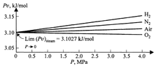
If we vary pressure ##P## and measure the corresponding values of volume ##V##, we can make a plot of ##P\frac{V}{n}=Pv## against ##P##.
This gives us some graph which has some form. Turns out that for a range of pressure starting at 0 the graph is approximately linear. At higher pressures, it becomes more nonlinear.
We can model this relationship using a power series
$$Pv=A(1+BP+CP^2+...)\tag{1}$$
Empirically, we see that for any such plot (ie, for any gas), the vertical intercept is the same. That is, ##A## is the same in the power series.
We can find what this limiting value is from the ideal gas law. For a constant volume gas, we have
$$T=273.16\text{K} \cdot \lim\limits_{P_{TP}\to 0} \left ( \frac{P}{P_{TP}} \right )\tag{2}$$
$$=273.16\text{K} \frac{\lim\limits_{P_{TP}\to 0} Pv}{\lim\limits_{P_{TP}\to 0} P_{TP}v}\tag{3}$$
and so
$$\lim\limits_{P_{TP}\to 0} Pv = \frac{\lim\limits_{P_{TP}\to 0} P_{TP}v}{273.16\text{K}}\cdot T\tag{4}$$
$$=RT$$
where $R$ is the molar gas constant.
We can also write
$$\lim\limits_{P_{TP}\to 0} PV=nRT\tag{5}$$
which is an equation of state for a gas in a hypothetical limit of low pressure.
Now, let's go back to the idea of modeling the entire relationship between ##Pv## and ##P##.
$$Pv=A(1+BP+CP^2+...)=RT(1+BP+CP^2+...)\tag{6}$$
$$\frac{Pv}{RT}=1+BP+CP^2+...\tag{7}$$
My question is about equation (7). Essentially, why is it interesting in this form?
Consider the following table

Here we have estimates for the virial coefficients in (7) for nitrogen gas.
Why is the formulation in (7) interesting?
Here is my attempt to answer this
- If the gas were ideal then we would have ##\frac{Pv}{RT}=1##. That is, ##B=C=D=...=0##.
- But we are dealing with a real gas.
- For a fixed temperature, if the value of ##\frac{Pv}{RT}## is above 1 then I assume this means that the molar volume is larger than expected for an ideal gas. I remember reading something in the past about intermolecular forces. Is this the origin of such a discrepancy at higher pressures?
- Below, I take the values of the table above for three temperatures and plot equation (7).

Thus, it seems that (7) allows us to gauge deviation from ideal gas behavior in a relatively simple way, namely deviation from 1.
If we vary pressure ##P## and measure the corresponding values of volume ##V##, we can make a plot of ##P\frac{V}{n}=Pv## against ##P##.
This gives us some graph which has some form. Turns out that for a range of pressure starting at 0 the graph is approximately linear. At higher pressures, it becomes more nonlinear.
We can model this relationship using a power series
$$Pv=A(1+BP+CP^2+...)\tag{1}$$
Empirically, we see that for any such plot (ie, for any gas), the vertical intercept is the same. That is, ##A## is the same in the power series.
We can find what this limiting value is from the ideal gas law. For a constant volume gas, we have
$$T=273.16\text{K} \cdot \lim\limits_{P_{TP}\to 0} \left ( \frac{P}{P_{TP}} \right )\tag{2}$$
$$=273.16\text{K} \frac{\lim\limits_{P_{TP}\to 0} Pv}{\lim\limits_{P_{TP}\to 0} P_{TP}v}\tag{3}$$
and so
$$\lim\limits_{P_{TP}\to 0} Pv = \frac{\lim\limits_{P_{TP}\to 0} P_{TP}v}{273.16\text{K}}\cdot T\tag{4}$$
$$=RT$$
where $R$ is the molar gas constant.
We can also write
$$\lim\limits_{P_{TP}\to 0} PV=nRT\tag{5}$$
which is an equation of state for a gas in a hypothetical limit of low pressure.
Now, let's go back to the idea of modeling the entire relationship between ##Pv## and ##P##.
$$Pv=A(1+BP+CP^2+...)=RT(1+BP+CP^2+...)\tag{6}$$
$$\frac{Pv}{RT}=1+BP+CP^2+...\tag{7}$$
My question is about equation (7). Essentially, why is it interesting in this form?
Consider the following table
Here we have estimates for the virial coefficients in (7) for nitrogen gas.
Why is the formulation in (7) interesting?
Here is my attempt to answer this
- If the gas were ideal then we would have ##\frac{Pv}{RT}=1##. That is, ##B=C=D=...=0##.
- But we are dealing with a real gas.
- For a fixed temperature, if the value of ##\frac{Pv}{RT}## is above 1 then I assume this means that the molar volume is larger than expected for an ideal gas. I remember reading something in the past about intermolecular forces. Is this the origin of such a discrepancy at higher pressures?
- Below, I take the values of the table above for three temperatures and plot equation (7).
Thus, it seems that (7) allows us to gauge deviation from ideal gas behavior in a relatively simple way, namely deviation from 1.