Cosmic inflation using mathematica

[Whitehole]

In cosmic inflation, we have the equation of motion for the inflaton given by,

$$\ddot\phi + 3H(1 + Q)\dot\phi + V_\phi = 0$$

the Friedman equation is given by

$$H^2 = \frac{1}{3 M_p^2}(\frac{1}{2} \dot\phi^2 + V + \rho_r)$$

where $M_p$ is the reduced Planck mass. The differential equation for the radiation density is given by

$$\dot\rho_r + 4H\rho_r = 3 Q H \dot\phi^2$$

Now for a given $V$, I want to solve these differential equations using NDSolve, let $V = \lambda (\phi^2 - \sigma^2)^2$

Let $\phi[t] = y[t]$, $\rho_r[t] = \rho[t]$, $Q=100$

Mp = 2.4353*10^18; (* Reduced Planck mass = 2.4353*10^18 GeV *)
m = 1.8*10^13; (* Inflaton mass = 1.8*10^13 GeV *)
Rm = (1.8*10^13 )/(2.4353*10^18); (* Rescaled inflaton mass *)
$\sigma$ = 2.24*10^19; (*Energy scale of symmetry breaking = 2.24*10^19 GeV*)
$R\sigma$ = (2.24*10^19)/(2.4353*10^18); (*Rescaled energy scale of symmetry breaking*)
$\lambda$ = ((1.8*10^13)/(2.4353*10^18))^4;
tf = 10^9;
sol[a_, b_] := NDSolve[{dy'[t] + 303 H[t] dy[t] + 4 \lambda (y[t]^2 - R\sigma^2) y[t] == 0, H[t] == Sqrt[(0.5 dy[t]^2 + \lambda (y[t]^2 - R\sigma^2)^2 + \rho[t])/3], \rho'[t] + 4 H[t] \rho[t] == 300 H[t] dy[t]^2, y'[t] == dy[t], y[0] == -a, dy[0] == b, \rho[0] == Rm^4}, {y, dy, H, \rho}, {t, 0, tf}]
sol[1, 1/100000]

This will generate interpolating functions. I need to determine the proper initial conditions $y[0] = -a$ and $tf$ ($dy[0] = b$, but it can be set to $10^{-6}$) for a fixed $Q$, in this case suppose I choose $Q=100$, so that I can get the correct values for the quantities.The initial conditions and $tf$ should be adjusted so that,

($N = \int Hdt$ where I represented $N$ by N1x in the code)
H[t] == Sqrt[(0.5 dy[t]^2 + \[Lambda] (y[t]^2 - R\[Sigma]^2)^2 + \[Rho][t])/3];
ndsol[a_, b_] := NDSolve[{D[N1x[t], t] == Evaluate[H[t] /. First@sol[a, b]], N1x[0] == 0}, N1x, {t, 0, tf}]

This plot should reach N1x = 60 after the plot/calculation,

Manipulate[Plot[Evaluate[N1x[t] /. First@ndsol[a, b]], {t, 0, tf}], {{a, 1}, 0, 100, Appearance -> "Labeled"}, {{b, 1/100000}, 0, 0.00009, Appearance -> "Labeled"}]

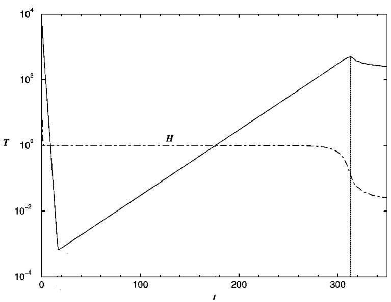
and the plot of $T$ vs. $t$ and $H$ vs $t$ generates a plot like the image below. ($~T = \Big(\frac{3 \rho_r}{10 \pi^2}\Big)^\frac{1}{4}$)
Manipulate[Plot[{Evaluate[H[t] /. First@sol[a, b]], Evaluate[(3 \[Rho][t]/10 Pi^2)^(1/4) /. First@sol[a, b]]}, {t, 0, tf}, PlotRange -> Automatic], {{a, 1}, 0, 50, Appearance -> "Labeled"}, {{b, 1/100000}, 0, 0.00009, Appearance -> "Labeled"}]

My code generates an error "For the method IDA, only machine real code is available. Unable to continue with complex values or beyond floating-point exceptions" for some $y[0] = -a$ and $tf$, so I'm having a hard time determining those two parameters. Actually, I don't know what tf to actually use, I'm just guessing. Is there a way to tell which $tf$ I should use so that the only thing I need to vary is $y[0]$?
A general rule for determining $y[0]$ is that it shouldn't be too far from the minimum of the potential $V$ but also not too close.

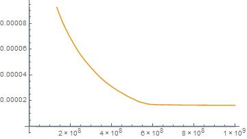
An example of my plot where $T \rightarrow yellow$ and $H \rightarrow blue$ (you can't even see it)

 

[NateD]

One way to determine the proper initial conditions and $tf$ is to use a numerical optimization algorithm. For example, you can use Mathematica's FindRoot command to find the roots of the equation N1x[tf] = 60, where N1x[tf] is the numerical solution for the integral of H with respect to t. This should give you the proper initial conditions for $y[0]$ and $tf$ that will produce the desired result. Another approach could be to use a simple brute force method of trying different values for $y[0]$ and $tf$ and seeing which ones give the desired result. However, this could take a long time and the results may not be very accurate.