- #1
superbread88
- 2
- 0
Have been trying for hours but simply no results. Hope that someone can help me out.
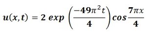
\[\frac{\partial u}{\partial t}=4\frac{\partial^2 u}{\partial x^2}\]
for \(t>0\) and \(0\leq x\leq 2\) subject to the boundary conditions
\[u_x (0,t) = 0\mbox{ and }u(2,t) = 0\]
and the initial condition
\[u(x,0) = 2 \cos \left(\frac{7\pi x}{4}\right)\]
By the use of separations of variables, solve the above equation for the temperature \(u(x,t)\)
Last edited by a moderator: