3D Schrödinger Equation for a magnetic vector potential in cylinder coordinates

[crazy-phd]

Hi there,
during my work on my PhD thesis as an experimental physicist I ended up with a very theoretical problem:
What does the wavefunction of an electron traveling through a magnetic vector potential look like?

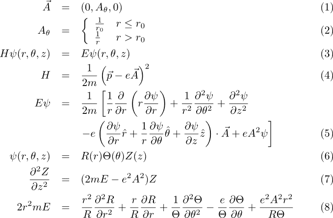
I chose a cylindrical coordinate system with a magnetic vector potential A (see eq (1) and (2)) for which I want to solve the Schrödinger equation (3). As there shall be no other potentials present the Hamilton operator looks like equation (4).

Using the considerations for the vector potential my differential equation looks like equation (5). In a first attempt I tried the usual separation of variables (equation (6)) which leads to two differential equations (7) and (8), in which R & Z and R & $\Theta$ are coupled.

Has anybody an idea on how to solve this "beast"?

Thank you

 

[hunt_mat]

I don't think that you have written an equation down that we can solve, you haven't said what is constant and what isn't. For example is E a constant?

If I get your notation, I think that (8) is wrong.

 

[crazy-phd]

Hi Mat,
as usual m,e and E are constants (mass, charge and kinetic energy of an electron).
I did not bother to insert for $A²$, but that would be equal to $1/r²$ or $1/r²_0$ ($r_0$ is an arbitrary constant].

If you have any other regards why equation (8) should be wrong, please let me know.

CU Andi

 

[hunt_mat]

Does your last term in (5) equal your last term in (8)? If that is the case and you are dividing through by $\psi$ then the last term in (8) should just be $eA^{2}$ (I think)

 

[crazy-phd]

It's me again.
After checking back to some books I decided to perform a Gauge Transformation of the form
$$\vec{A}' = \vec{A}+\mathrm{grad}\Lambda=0$$
such that the solution to the initial Schrödinger equation becomes
$$\psi = \psi'*\mathrm{e}^{\frac{ie}{\hbar c}\Lambda},$$
where $\psi'$ is the solution of the Schrödinger equation in the absence of a magnetic vector potential, i is the complex number.

In order to got to my desired solution I have to solve a much simpler differential equation
$$\vec{A} = \vec{\nabla}\Lambda$$.
Due to symmetries of my problem - as mention in the previous post - the vector A looks in a more difficult form like this in cylindrical coordinates:
$$\vec{A}=\left(A_r,\,A_\theta,\,A_z\right),\; A_r=\left\{\begin{array}{cc}\propto r & r<r_0\\ \propto\frac{1}{r} & r>r_0\end{array}\right.,\,A_\theta=\theta+\frac{1}{2}\pi,\,A_z=0$$

Thanks to "trial and error" I can consider a good approximation for $\Lambda$ for the last case $r>r_0$ to be the following
$$\Lambda(r,\,\theta,\,z)\propto\pi\theta+\theta^2$$

My remaining problem now is the first case. What does $\Lambda$ look for $r<r_0$?
Can anybody suggest an analytical or numeric solution??

Thank you

 

[hunt_mat]

A has to be continuous at $r=r_{0}[/itex}? Then just integrate. You should have one boundary condition and one matching condition for the two constants.$

 

[crazy-phd]

That's exactly what I thought when I started out with this adventure: "just" integrate.

Yes, it would be helpful for $\Lambda$ to be continuous at $r=r_0$

But one has to keep in mind, that I'm talking about a 3 dimensional vector potential $\vec{A}$ and a scalar function $\Lambda$ of 3 variables. So I end up with a set of differential equations:
$$\begin{eqnarray}<br /> \frac{\partial\Lambda(r,\,\theta,\,z)}{\partial r} &=& A_r = \left\{\begin{array}{cc}k_1r & r<r_0\\ k_2\frac{1}{r} & r>r_0\end{array}\right.,\; k_i: \mathrm{constants}\\<br /> \frac{1}{r}\frac{\partial\Lambda(r,\,\theta,\,z)}{\partial\theta} &=& A_\theta=\theta+\frac{\pi}{2}\\<br /> \frac{\partial\Lambda(r,\,\theta,\,z)}{\partial z} &=& A_z = 0<br /> \end{eqnarray}$$

As mentioned previously the case $r>r_0$ is almost trivial. The problem is one has to find a scalar function $\Lambda(r,\,\theta)$ that solves the first two equations. None of the expressions I tried as a solution for $\Lambda(r,\,\theta)$ did reconstruct the initial $\vec{A}$.

I tried several forms of "separation of variables", but none resulted in a solution.
This is why I am asking for help in this forum...

 

[hunt_mat]

From the third equation you know that $\Lambda =\Lambda (r,\theta )$, from the second equation you find that:
$$\Lambda =\frac{1}{2}r\theta^{2}+f(r)$$
Where f(r) is an arbitrary function of r. and if you plug this into the first equation you find that:
$$\frac{1}{2}\theta^{2}+f'(r)=\left\{<br /> \begin{array}{cc}<br /> k_{1}r & r<r_{0} \\<br /> \frac{k_{2}}{r} & r>r_{0}<br /> \end{array}\right.$$
Can you integrate that?

 

[crazy-phd]

Your equations can be solved without big problems:
$$\Lambda(r,\,\theta,\,z) = \frac{1}{2}r\theta^2+\left\{\begin{array}{cc}<br /> \frac{2k_1\mathrm{ln}(r)}{\theta(\theta+\pi)} & r>r_0\\<br /> \frac{k_2r^2}{\theta(\theta+\pi)} & r<r_0<br /> \end{array}\right.$$
The gradient of this expression does not show a similar behavior like the initial vector potential, which suggests that this is no true solution to the equation.

This is a cut plane through the original vector potential.

This is $\Lambda$ in the z=0 plane.

This is the gradient of $\Lambda$, which shows clearly a different behavior.

Using another approach
$$\Lambda(r,\,\theta,\,z)=\left\{\begin{array}{cc}<br /> \frac{1}{2}\theta^2+\pi\theta & r>r_0\\<br /> ? & r<r_0<br /> \end{array}\right.$$

This results in a similar behavior for $r>r_0$. In the following figure $\vec{\nabla}\Lambda$ is plotted for the entire range of r.

 

[hunt_mat]

Looking that the solution you gave, I don't think you've got the correct solution as you have a singularity at $\theta =0,-\pi$ and when you set $r=r_{0}$ you don't get the same solution.

Also looking at your initial equations, $A_{\theta}$ appears to be constant for $r<r_{0}$ and yet in your later equations it isn't. I don't think that you've solved the equations correctly.

 

[pschatt]

You cannot get rid of the vector potential with your gauge transformation because A has non-vanishing rotation. The problem has been solved in 1928 by Fock. Solutions of the radial part are associated Laguerre polynomials. See S. Mikhailov, Physica B 299 (2001), 6-31