"Barlow's wheel" used as an electrical generator

[Ale_Rodo]

In this thread, I hope to find some help in understanding one of the first application of Faraday's law of induction: the "Barlow's wheel".

Basically the machine converts electrical power to mechanical, so as you can imagine, a battery, some conductor wires, a horseshoe magnet and a metal wheel are required for this set up.
---Note: The wheel used by my professor was circular, basically a disk and not a star-shaped wheel as you might find on the internet.

CASE 1: (electric -> mechanical)
We connect the battery to the wheel in such a way that current will flow unless the switch is OFF (mercury as a contact might be needed, but it's just a 'real life experiment' need, I believe). The metal wheel must be standing on some support and has to be placed in between the two horseshoe magnet's poles so that we have some flux of magnetic field through a part of the wheel.

Now, when we close the circuit (ON), a current will flow through the wheel passing by the magnetic field, so a Lorentz force will act on every and each particle moving in that region causing a torque on the wheel, which will start spinning with an angular velocity.

CASE 2: (mechanical -> electric)
Same setup (except we don't want to connect the battery this time), but now we want to convert mechanical power to electrical by spinning the wheel manually with the help of a handle.
From what I understood of my professor's lecture, this should induce an e.m.f. in the circuit, achieving the goal, but I can't understand how this is possible, since I thought that a change in magnetic flux through time must happen and the wheel doesn't increase nor decrease the surface area where the flux, well..."flows".

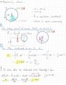
I'll attach a screenshot of what I copied about my professor's notes ('copied', because I didn't understand).

Thank you in advance for your answers.

 

[phyzguy]

If you look at Feynman's lectures at this link, he discusses this case in the section "Exceptions to the flux rule", and explains why you have to be careful blindly applying the flux rule.

 

[vanhees71]

If I remember right, Feynman does not mention that in reality there is no exception to the flux rule. What's always valid are the Maxwell equations in differential (local) form. Here we have Faraday's Law (in SI units),
$$\vec{\nabla} \times \vec{E}=-\partial_t \vec{B}.$$
Then integrating this equation over an arbitrary surface (which may be time dependent) leads to
$$\int_{\partial A} \mathrm{d} \vec{r} \cdot \vec{E}(t,\vec{r}) = -\int_A \mathrm{d}^2 \vec{f} \cdot \vec{B}(t,\vec{r}).$$
Now the critical issue is, how to draw the time-derivative out of the integral. If $A$ is time-independent you can simply commute integration and differentiation, while for a time-dependent surface you have to take into account that the time derivative also acts on the integration region, and in fact it should not.

In continuum mechanics that's known as "Reynolds's transport theorems". The one for surface integrals for arbitrary vector fields and arbitrarily moving surfaces it reads
$$\mathrm{d}_t \int_A \mathrm{d}^2 \vec{f} \cdot \vec{V}(t,\vec{r}) = \int_A \mathrm{d}^2 \vec{f} \cdot [\partial_t \vec{V}(t,\vec{r}) + \vec{v} (\vec{\nabla} \cdot \vec{V}(t,\vec{r}))] - \int_{\partial A} \mathrm{d} \vec{r} \cdot (\vec{v}(t,\vec{r}) \times \vec{V}(t,\vec{r}),$$
where $\vec{v}(t,\vec{r})$ is the velocity of the points along the surface.

For $\vec{B}$ we have $\nabla \cdot \vec{B}=0$ and thus
$$\mathrm{d}_t \int_A \mathrm{d}^2 \vec{f} \cdot \vec{B}=\int_A \mathrm{d}^2 \vec{f} \partial_t \vec{B} - \int_{\partial A} \mathrm{d} r \cdot (\vec{v} \times \vec{B}).$$
Thus we have
$$\int \mathrm{d}^2 \vec{f} \partial_t \vec{B}=\mathrm{d}_t \int_{A} \mathrm{d}^2 \vec{f} \cdot \vec{B} + \int_{\partial A} \mathrm{d} r \cdot (\vec{v} \times \vec{B}).$$
For Faraday's Law this means (combining the two line integrals to the complete electromotive force on the left-hand side),
$$\mathcal{E}=\int_{\partial A} \mathrm{d} \vec{r} \cdot (\vec{E} + \vec{v} \times \vec{B}) = -\mathrm{d}_t \int_A \mathrm{d}^2 \vec{f} \cdot \vec{B}=-\dot{\Phi}_B.$$

 

[phyzguy]

@vanhees71 , I don't understand your argument. In the case of Feynman's Figure 17-2, A is not time dependent. It is a fixed region in space. The flux through this region does not change with time. Yet there is an EMF.

 

[etotheipi]

If the surface $A$ is time-independent then it's even easier because then you can just pull the $\frac{\partial}{\partial t}$ outside of the integral without including any correction terms,\begin{align*}
\int_A (\nabla \times \mathbf{E}) \cdot d\mathbf{S} = - \int_A \frac{\partial \mathbf{B}}{\partial t} \cdot d\mathbf{S} \implies \int_{\partial A} \mathbf{E} \cdot d\mathbf{r} = - \frac{d}{dt} \int_A \mathbf{B} \cdot d\mathbf{S}
\end{align*}It's only if $A = A(t)$ that you need to use the Reynold's transport theorem [generalisation of the Leibnitz integral rule] and in such cases there is also a $\int (\mathbf{v} \times \mathbf{B}) \cdot d\mathbf{r}$ contribution to $\mathcal{E}$

 

[phyzguy]

If the surface $A$ is time-independent then it's even easier because then you can just pull the $\frac{\partial}{\partial t}$ outside of the integral without including any correction terms,\begin{align*}
\int_A (\nabla \times \mathbf{E}) \cdot d\mathbf{S} = - \int_A \frac{\partial \mathbf{B}}{\partial t} \cdot d\mathbf{S} \implies \int_{\partial A} \mathbf{E} \cdot d\mathbf{r} = - \frac{d}{dt} \int_A \mathbf{B} \cdot d\mathbf{S}
\end{align*}It's only if $A = A(t)$ that you need to use the Reynold's transport theorem [generalisation of the Leibnitz integral rule] and in such cases there is also a $\int (\mathbf{v} \times \mathbf{B}) \cdot d\mathbf{r}$ contribution to $\mathcal{E}$

Right. But the whole point of Feynman's discussion is that in this case the RHS (d/dt of flux of B through the loop) is zero, but the LHS (EMF) is not.

 

[etotheipi]

It's an interesting example because I think there's a few different approaches you can take. For example, first let $\partial A = \partial A(t)$ everywhere move with the same velocity as the conductor. For instance in Fig. 17-2 we may write $\partial A(t) = C_1(t) \cup C_2$ where $C_1(t)$ is a curve that at time $t_0$ instantaneously connects the centre of the disc to the top-most point of the disc, and $C_2$ is the curve which follows the wire to the galvanometer, then back to the axle and returns to the start point of $C_1$ at the centre of the disc. Then you can write $$\mathcal{E} = \int_{\partial A(t)} (\mathbf{E} + \mathbf{v} \times \mathbf{B}) \cdot d\mathbf{r} = -\frac{d}{dt} \int_{A(t)} \mathbf{B} \cdot d\mathbf{S}$$except here the right hand side does not vanish because $A(t)$ depends on time whilst $\mathbf{B}(\mathbf{r})$ does not depend on time. So I don't think this equation is very useful here, at least not operationally.

The alternative approach would be to let $\partial B = \tilde{C}_1 \cup C_2$ be a time-independent curve with $\tilde{C}_1$ stationary and connecting the centre of the disc to the top-most point, and $C_2$ as before. Then write\begin{align*}
\int_{\partial B} \mathbf{E} \cdot d\mathbf{r} &= - \underbrace{ \frac{d}{dt}\int_B \mathbf{B} \cdot d\mathbf{S}}_{=\, 0} \\

\int_{\partial B} \mathbf{E} \cdot d\mathbf{r} + \int_{\partial B} (\mathbf{v} \times \mathbf{B}) \cdot d\mathbf{r} &= \int_{\partial B} (\mathbf{v} \times \mathbf{B}) \cdot d\mathbf{r} \\ \\

\mathcal{E} &= \int_{\partial B} (\mathbf{v} \times \mathbf{B}) \cdot d\mathbf{r}
\end{align*}where here we are careful to note that $\mathbf{v}$ is the velocity of the conducting material. Does that look okay to you, @vanhees71?

 

[vanhees71]

@vanhees71 , I don't understand your argument. In the case of Feynman's Figure 17-2, A is not time dependent. It is a fixed region in space. The flux through this region does not change with time. Yet there is an EMF.

Yes, this is a variant of the homopolar generator, and there the solution is that if you want to stick to standard macroscopic electrodynamcis you have to use the correct relativistic Ohm's Law, which takes correctly into account the Hall effect, and this is of course derived from microscopic electrodynamics exactly as Feynman explains from first principles using the Lorentz force on the conduction electrons. Nevertheless there are no exceptions to Faraday's Law, which is one of the fundamental Maxwell equations. The treatment of this often confusing issue in Feynman vol. II is excelenct, but I think the correct derivation of the complete integral form of Faraday's law is not given there.