MHB How does tikx help to create graphs for a car's motion?

[karush]

from tikx package...

\begin{tikzpicture}
%\draw (0,5) -- (6,5);
\draw [thick] (0,1) -- (18/2,1);
\node at (0,.8){0};
\node at (18/2,.8){180};
%\draw (1,5)--(1,4)--(2,4);
%\node at (1.5,4.1) {v};
\draw[step=.45 cm,gray,very thin,dashed]
%(-6,0)
grid (18/2,8);
\end{tikzpicture}

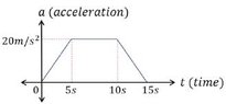
At $t=0$ a car is stopped at a traffic light
When the light turns green, the car starts to speed up,
and gains speed at a constant rate until it reaches a speed of $2 m/s \, 8s$ after the light turns green.
The car continues at a constant speed for $60m$
Then the driver sees a read light up ahead at the next intersection, and starts slowing down at a constant rate.
The car stops at the red light, $180 m$ form where it was at $t=0$a) Draw $x_t, v_t,$ and $a_t$ graphs for the motion of the car
b) In a motion diagram show the position, velocity and acceleration of the car.ok I am tying to do this using tikx but got stuck at the beginingI currently have the x-axis at distance but maybe it shud be time
we might need actually 2 graphs

I think the velocity is really $2m/s$
$v = v_0 + at$
then
$\dfrac{v-v_0}{t}=a$
so
$\dfrac{2m/s}{s}=\dfrac{2m}{s^2}=a$

 

[HallsofIvy]

If you have the x-axis as distance, what is the y-axis? I suggest that the x-axis be t, time, and the x-axis be the distance traveled in that time. At constant speed the graph is a straight line, at constant acceleration or deceleration the graph is a parabola.

 

[karush]

why would a constant acceleration be a parabola the slope doesn't change

I think one graph a-t would be the one I should do

here is sample from another problem from google images

View attachment 9249

 

[I like Serena]

The speed of $2\text{ m/s}$ seems rather low for a car — it's a walking speed.

Either way, we could for instance draw the graphs like this:
\begin{tikzpicture}[xscale=0.2,yscale=.04]
%preamble \usepackage{amsmath}
\draw[xstep=2,ystep=10,lightgray,very thin] (0,-20) grid (150,260);
\draw (8,0) -- (8,250) (38,-18) -- (38,100) (150,-18) -- (150,180);
\draw[thick,->] (0,0) node[below] {0 s} -- (8,0) node[below] {8 s} -- (38,0) node[below] {38 s} -- (150,0) node[below] {150 s} -- (155,0) node

{$t$};
\draw[thick,->] (0,0) -- (0,260);
\draw[ultra thick,red] (0,250) -- node[below] {$a_t$} (8,250) node

{$0.25\text{ m/s}^2$} -- (8,0) -- (38,0) -- (38,-18) node

{$-0.018\text{ m/s}^2$} -- (150,-18);
\draw[ultra thick,cyan] (0,0) -- node[above left] {$v_t$} (8,100) node

{2 m/s} -- (38,100) node[above] {2 m/s} -- (150,0);
\draw[ultra thick,blue] (0,0) parabola (8,8) node[above left] {8 m} -- node[above left] {$x_t$} (38,68) node[below right] {68 m} parabola bend (150,180) (150,180) node[above] {180 m};
\end{tikzpicture}​

 

[karush]

yeah I think it should be 20 not 2
the copy was really hard to read...
that would make the horizontal lite blue line to 8+3=11s
wow thanks for the graph

ok I did this fot a-t and 20 m/s

\begin{tikzpicture}[xscale=0.2,yscale=.04]
%preamble \usepackage{amsmath}
\draw[xstep=2,ystep=10,lightgray,very thin] (0,0) grid (40,160);
%\draw (8,0) -- (8,250) (38,-18) -- (38,100) (150,-18) -- (150,180);
\draw[thick,->]
(0,0) node[below] {0 s}
-- (16,0) node[below] {8 s} -- (11*2,0) node[below] {11 s} -- (15*2,0) node[below] {15 s} -- (40,0) node

{$t$};
\draw[thick,->] (0,0)-- (0,100) node

{20 m/s} -- (0,160);
%\draw[ultra thick,red] (0,250) -- node[below] {$a_t$} (8,250) node

{$0.25\text{ m/s}^2$} -- (8,0) -- (38,0) -- (38,-18) node

{$-0.018\text{ m/s}^2$} -- (150,-18);
\draw[ultra thick,cyan] (0,0) -- node[above left] {$v_t$} (8*2,100) -- (11*2,100) -- (30,0);

% \draw[ultra thick,blue] (0,0) parabola (8,8) node[above left] {8 m} -- node[above left] {$x_t$} (38,68) node[below right] {68 m} parabola bend (150,180) (150,180) node[above] {180 m};
\end{tikzpicture}

clueless about the speed parabola​