How to interpret Cost Function?

In summary, the conversation discusses the interpretation of the cost function in machine learning and how the values of theta zero and theta one affect the slope of a straight line on a graph. It is explained that theta one does not have units and represents the increase in the vertical coordinate for every unit increase in the horizontal coordinate. The conversation also includes an exercise to plot different lines on a graph to better understand the concept.
  • #1
Richard_Steele
53
3
I am just starting a course about machine learning and I don't know how to interpret the cost function.
2j2i5aq.jpg


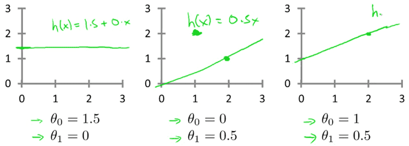
When the teacher draws the straight line in the x and y coordinates, it looks like:
1491kcg.jpg


I see that theta zero is the start of the straight line (in the left side) in the Y coordinate.
The question is related about what theta one modifies? theta one modifies the inclination?
 
Physics news on Phys.org
  • #2
Richard_Steele said:
The question is related about what theta one modifies? theta one modifies the inclination?
Yes, also called the slope.

However, how this is to be interpreted in a machine learning context is not clear to me, as I never really understood what that field is about. EDIT: Maybe somebody such as @StatGuy2000 can help you with the interpretation?
 
Last edited:
  • Like
Likes Richard_Steele
  • #3
Krylov said:
Yes, also called the slope.

However, how this is to be interpreted in a machine learning context is not clear to me, as I never really understood what that field is about.
Of course, so Theta_1 modifies the slope.
But, I don't interpret the measuring scale of the slope. In the examples (middle and right, the graphs I posted on post #1), Theta_1 = 0.5.
What kind of unit is 0.5? Degrees? I don't know how to interpret 0.5 with the slope of the straight line.

Responding to your question about machine learning, this algorithm is used in linear regression. You give a dataset to your algorithm (example: x=house's size and y=price of the house), and you have to calculate a straight line that better fits to your dataset. Then, you give to the algorithm values of X (size of the house) and the software calculates the value of Y (price of the house). This is used in supervised learning. Supervised means that you give the correct answers to the software and the software can learns from data. Unsupervised learning means that you give data to the software, but nos classified data (no correct answer given in the data).
 
  • #4
I moved the thread to our homework section, as it is homework-like.

Richard_Steele said:
What kind of unit is 0.5? Degrees?
It does not have units. It means if x (the horizontal coordinate) increases by 1, then h (the vertical coordinate) increases by 0.5. You can see that if you check the function definition and increase x by 1.
 
  • Like
Likes EnumaElish and Richard_Steele
  • #5
Richard_Steele said:
I am just starting a course about machine learning and I don't know how to interpret the cost function.
2j2i5aq.jpg


When the teacher draws the straight line in the x and y coordinates, it looks like:
1491kcg.jpg


I see that theta zero is the start of the straight line (in the left side) in the Y coordinate.
The question is related about what theta one modifies? theta one modifies the inclination?

Just look at the three diagrams. What do you see when you compare the first two? To anchor your understanding, try the following little exercise for yourself: plot the line y=1+x, which uses ##\theta_0=1, \theta_1=1##. Compare that new line with the third line plotted above. What do you see?
 
  • Like
Likes Richard_Steele
  • #6
Ray Vickson said:
Just look at the three diagrams. What do you see when you compare the first two? To anchor your understanding, try the following little exercise for yourself: plot the line y=1+x, which uses ##\theta_0=1, \theta_1=1##. Compare that new line with the third line plotted above. What do you see?
I see that the point where the straight line passes through Y is 1 (Y=1). When it increases X in 1 unit, then Y = X + 1, so Y is always one unit higher than X.
Right?
 
  • #7
Richard_Steele said:
I see that the point where the straight line passes through Y is 1 (Y=1). When it increases X in 1 unit, then Y = X + 1, so Y is always one unit higher than X.
Right?

Yes, but I asked you to compare the new line with the third line given in post #1. Take a sheet of graph paper; plot both lines on the same sheet. Now tell me what you see.
 
  • #8
Ray Vickson said:
Just look at the three diagrams. What do you see when you compare the first two? To anchor your understanding, try the following little exercise for yourself: plot the line y=1+x, which uses ##\theta_0=1, \theta_1=1##. Compare that new line with the third line plotted above. What do you see?
2zyy4aw.jpg
 
  • #9
Ray Vickson said:
Yes, but I asked you to compare the new line with the third line given in post #1. Take a sheet of graph paper; plot both lines on the same sheet. Now tell me what you see.
Ok, in a few minutes you will have here the comparations.
 
  • #10
Ray Vickson said:
Yes, but I asked you to compare the new line with the third line given in post #1. Take a sheet of graph paper; plot both lines on the same sheet. Now tell me what you see.

I see a variation in the slope. The 1 + 1X has more slope than 1 + 0.5X
14wwplf.jpg
 
  • #11
Richard_Steele said:
I see a variation in the slope. The 1 + 1X has more slope than 1 + 0.5X
14wwplf.jpg

Exactly. When x increases by 1, 1+x increases by 1 but 1 + .5*x increases by 1/2.

It would have been more revealing if you had (as I suggested) plotted both lines on the same sheet of paper. If the software you are using does not allow that, then do it by hand on an actual, physical sheet of paper. Alternatively, you can use the graphing packages in a typical spreadsheet to plot several lines or curves on the same plot.
 
  • Like
Likes Richard_Steele
  • #12
Ray Vickson said:
Exactly. When x increases by 1, 1+x increases by 1 but 1 + .5*x increases by 1/2.

It would have been more revealing if you had (as I suggested) plotted both lines on the same sheet of paper. If the software you are using does not allow that, then do it by hand on an actual, physical sheet of paper. Alternatively, you can use the graphing packages in a typical spreadsheet to plot several lines or curves on the same plot.
Graphs plotted on sheet of paper.
1zezr5.jpg
 
  • #13
Richard_Steele said:
Graphs plotted on sheet of paper.
1zezr5.jpg

Good; that really does show up the difference most dramatically.
 
  • Like
Likes Richard_Steele
  • #14
Ray Vickson said:
Good; that really does show up the difference most dramatically.
Yes, it's more clear when I draw both on the same graph.

I am reading about 'minimizing the cost function'. What means minimizing and why is minimization used?
 
  • #15
Richard_Steele said:
Yes, it's more clear when I draw both on the same graph.
Your graphs ought to show the equations; that is, y = 1 + x and y = 1 + 0.5x.

Also, the axes are usually labelled on the positive ends. You have your labels for the x-axis on the negative end.
Richard_Steele said:
I am reading about 'minimizing the cost function'. What means minimizing and why is minimization used?
Any business that manufactures and sells a product is always interested in maximizing its profit. One way to do this is to minimize (make as small as possible) its costs.
 
  • Like
Likes Richard_Steele
  • #16
Mark44 said:
Your graphs ought to show the equations; that is, y = 1 + x and y = 1 + 0.5x.

Also, the axes are usually labelled on the positive ends. You have your labels for the x-axis on the negative end.

Any business that manufactures and sells a product is always interested in maximizing its profit. One way to do this is to minimize (make as small as possible) its costs.
Thanks for the advices.

I am learning cost function applied to machine learning. I am using it in linear regression. So I don't know if minimization has the same objective in manufacturing and in machine learning.
 
  • #17
Richard_Steele said:
I am learning cost function applied to machine learning. I am using it in linear regression. So I don't know if minimization has the same objective in manufacturing and in machine learning.
I don't know how it's related to machine learning, but maybe how long it takes for a program to learn something? Maybe that's what "cost" means in this situation.
 
  • #18
Mark44 said:
I don't know how it's related to machine learning, but maybe how long it takes for a program to learn something? Maybe that's what "cost" means in this situation.
In the video, the teacher is showing a cartesian plane. Horizontal line, X, is the size of the house. Vertical line, Y, is the price of the house. That dataset is called 'the training set' (it contains the correct answers).

Then, with the training set, the program has to calculate the straight line I was asking about in the #1 post in this thread. Of course, after that, its needed to 'minimize the function'. It's something like calculating the best parameters for theta zero and theta one, to produce a straight line that minimizes the error between the Y values (those from the trained dataset) and the h(x) (the hypothesis, the predicted Y value). This predicted Y value is called the prediction or the hypothesis. The only real Y values come from the real dataset (the training dataset).

The question is what minimization does and why we should apply it.
 
  • #19
mfb said:
I moved the thread to our homework section, as it is homework-like.

It does not have units. It means if x (the horizontal coordinate) increases by 1, then h (the vertical coordinate) increases by 0.5. You can see that if you check the function definition and increase x by 1.
The slope parameter is measured in Y units/X units. In the equation Y = a + b X, b = ∂Y/∂X. If Y is "meters traveled" and X is "seconds of time" then b corresponds to velocity measured in meters per second. (In an estimation context b would be called average velocity or average incremental distance.) If Y is dollars and X is square feet then b is the increase in dollars when area increases 1 sqft. In this case b is measured in dollars per sqft.
 
Last edited:
  • Like
Likes Richard_Steele
  • #20
EnumaElish said:
In the equation Y = a + b X, b = ∂Y/∂X
Where Y is a function of one variable, X, the slope would be dY/dX. Of course, in the case, the partial you wrote would be the same as the derivative I wrote. However, as this thread is in the Precalc section, the OP might not be familiar with derivatives of any kind.
 
  • #21
Richard_Steele said:
In the video, the teacher is showing a cartesian plane. Horizontal line, X, is the size of the house. Vertical line, Y, is the price of the house. That dataset is called 'the training set' (it contains the correct answers).

Then, with the training set, the program has to calculate the straight line I was asking about in the #1 post in this thread. Of course, after that, its needed to 'minimize the function'. It's something like calculating the best parameters for theta zero and theta one, to produce a straight line that minimizes the error between the Y values (those from the trained dataset) and the h(x) (the hypothesis, the predicted Y value). This predicted Y value is called the prediction or the hypothesis. The only real Y values come from the real dataset (the training dataset).

The question is what minimization does and why we should apply it.

Since no line will fit the data exactly, when can we say that one fit is better, or more accurate than another on average? People have devised several measures of error, and the oldest one (which has been around for centuries) is the so-called squared-error measure. If you have a data set ##(x_1,y_1), (x_2,y_2), \ldots, (x_n,y_n)## and plot them (as a set of point in xy-space), you might get the feeling that the points should lie on or near a straight line of the form ##y = a + bx##. If somebody tells you values of the intercept ##a## and the slope ##b##, you can calculate the "fitted" values of y, which are ##a + b x_i## for ##i = 1,2 \ldots, n##. In general, some of the fitted values will not agree with the experimental (or observed) values of ##y## at the same ##x##-points, so we will have some errors ##e_i = a + b x_i - y_i## for ##i = 1,2, \ldots, n##.

We would like to measure the "goodness" of the fit by forming some kind of aggregate error measure that depends on all the values of ##e_i##. The (total) squared-error criterion is ##S_2 = e_1^2 + e_2 ^2 + \cdots + e_n^2##. Because the errors are squared, they contribute the same whether they are > 0 or < 0, and again because they are squared, large error values make more of a contribution to the total than do small errors. For example, if ##e_2 = 10 e_1## then ##e_2^2 = 100 e_1^2##, so in a sense, ##e_2## is a hundred times more crucial or important than is ##e_1##.

Anyway, regardless of the justification, the measure ##S_2## as above is one of the standard measures used in making data fits; it is the oldest historically and the easiest to use.

To find a "best" fit in the total squared error sense, we would like to find parameters ##a## and ##b## that make the value of ##S_2## as small as possible. That is, we want to minimize ##S_2##. Because the errors are squared, when we minimize ##S_2## we are trying hard to avoid really large errors.

In recent times, alternative error measures have been proposed, and they sometimes have better properties than ##S_2##. For example, the least-total deviation fit determines ##a## and ##b## so as to minimize the total absolute error ##S_1 = |e_1| + |e_2| + \cdots + |e_n|##. Determining the best ##a,b## values in this case is more involved than in the squared-error case, and is best attacked using the relatively modern tools of linear programming (invented in the late 1940s or early 1950s, essentially). Minimizing ##S_1## can lead to fits that are more tolerant of "outliers", so one or two individual "bad" data points (that can throw off the least-squares fit badly) are de-emphasized in the least-deviation fit; it is almost as though the least-deviation method is smart enough to ignore really, really bad points.

Anyway, those are the kinds of things we aim to minimize, and we do so to try to make the fit as accurate as possible, knowing that 100% accuracy is impossible.
 
  • Like
Likes Richard_Steele
  • #22
Ray Vickson said:
Since no line will fit the data exactly, when can we say that one fit is better, or more accurate than another on average? People have devised several measures of error, and the oldest one (which has been around for centuries) is the so-called squared-error measure. If you have a data set ##(x_1,y_1), (x_2,y_2), \ldots, (x_n,y_n)## and plot them (as a set of point in xy-space), you might get the feeling that the points should lie on or near a straight line of the form ##y = a + bx##. If somebody tells you values of the intercept ##a## and the slope ##b##, you can calculate the "fitted" values of y, which are ##a + b x_i## for ##i = 1,2 \ldots, n##. In general, some of the fitted values will not agree with the experimental (or observed) values of ##y## at the same ##x##-points, so we will have some errors ##e_i = a + b x_i - y_i## for ##i = 1,2, \ldots, n##.

We would like to measure the "goodness" of the fit by forming some kind of aggregate error measure that depends on all the values of ##e_i##. The (total) squared-error criterion is ##S_2 = e_1^2 + e_2 ^2 + \cdots + e_n^2##. Because the errors are squared, they contribute the same whether they are > 0 or < 0, and again because they are squared, large error values make more of a contribution to the total than do small errors. For example, if ##e_2 = 10 e_1## then ##e_2^2 = 100 e_1^2##, so in a sense, ##e_2## is a hundred times more crucial or important than is ##e_1##.

Anyway, regardless of the justification, the measure ##S_2## as above is one of the standard measures used in making data fits; it is the oldest historically and the easiest to use.

To find a "best" fit in the total squared error sense, we would like to find parameters ##a## and ##b## that make the value of ##S_2## as small as possible. That is, we want to minimize ##S_2##. Because the errors are squared, when we minimize ##S_2## we are trying hard to avoid really large errors.

In recent times, alternative error measures have been proposed, and they sometimes have better properties than ##S_2##. For example, the least-total deviation fit determines ##a## and ##b## so as to minimize the total absolute error ##S_1 = |e_1| + |e_2| + \cdots + |e_n|##. Determining the best ##a,b## values in this case is more involved than in the squared-error case, and is best attacked using the relatively modern tools of linear programming (invented in the late 1940s or early 1950s, essentially). Minimizing ##S_1## can lead to fits that are more tolerant of "outliers", so one or two individual "bad" data points (that can throw off the least-squares fit badly) are de-emphasized in the least-deviation fit; it is almost as though the least-deviation method is smart enough to ignore really, really bad points.

Anyway, those are the kinds of things we aim to minimize, and we do so to try to make the fit as accurate as possible, knowing that 100% accuracy is impossible.
Just reading your post. It will take time to digest all the information. I will ask you as soon as I finish reading everything.
 
  • #23
Ray Vickson

So let's start little by little... let's talk about the first paragraph.
Lets think we have a dataset ##(X_1,Y_1), \ldots, (X_n, Y_n)##. As you said, it is possible that those points in the xy space form groups. So our task is to find a straight line that is like the 'mean' of those points.

I am going to try to explain it better.
2qwg0sl.jpg

Imagine that we have that cloud of points, so we have to calculate the ##y= a + bx## (the straight line). What happens while calculating the straight line? The problem here is that we have to calculate ##a## and ##b## values to get a straight line that contains the lower amount of errors.

But, what is an error?
We know that is impossible to get a straight line that represents with 100% accuracy all the ##x,y## points in the graph.
A "perfect" case would be this one:
2jeskuc.jpg

It's perfect (without errors), because all the points belong to the straight line. So any prediction that we would do, givin an ##x_n## value, will output an exact ##Y## value, without errors.
The problem starts when we have some "errors", like this one:
v4pdts.jpg

The green (I have used green to make it easier to differentiate) points are not fitted to the straight line. Using linear algebra it's impossible to create a straight line that contains all the points of the graph. So, when we try to predict ##Y## values, the output won't be 100% accurate because it will contain some error percentage.
An error will be the next:
wkh3rs.jpg

Because the predicted value doesn't represent the real value. There is an error between the ##real value## and the ##predicted value##.
If we analyze a huge amount of points, there will be a huge amount of errors, right?

So our task is to calculate the straight line that contains the lower amount of errors, right? For that reason, it's called "minimization", because we are trying to minimize the total amount of errors, right?
 
  • #24
Richard_Steele said:
Ray Vickson

So let's start little by little... let's talk about the first paragraph.
Lets think we have a dataset ##(X_1,Y_1), \ldots, (X_n, Y_n)##. As you said, it is possible that those points in the xy space form groups. So our task is to find a straight line that is like the 'mean' of those points.

I am going to try to explain it better.
2qwg0sl.jpg

Imagine that we have that cloud of points, so we have to calculate the ##y= a + bx## (the straight line). What happens while calculating the straight line? The problem here is that we have to calculate ##a## and ##b## values to get a straight line that contains the lower amount of errors.

But, what is an error?
We know that is impossible to get a straight line that represents with 100% accuracy all the ##x,y## points in the graph.
A "perfect" case would be this one:
2jeskuc.jpg

It's perfect (without errors), because all the points belong to the straight line. So any prediction that we would do, givin an ##x_n## value, will output an exact ##Y## value, without errors.
The problem starts when we have some "errors", like this one:
v4pdts.jpg

The green (I have used green to make it easier to differentiate) points are not fitted to the straight line. Using linear algebra it's impossible to create a straight line that contains all the points of the graph. So, when we try to predict ##Y## values, the output won't be 100% accurate because it will contain some error percentage.
An error will be the next:
wkh3rs.jpg

Because the predicted value doesn't represent the real value. There is an error between the ##real value## and the ##predicted value##.
If we analyze a huge amount of points, there will be a huge amount of errors, right?

So our task is to calculate the straight line that contains the lower amount of errors, right? For that reason, it's called "minimization", because we are trying to minimize the total amount of errors, right?

Yes, but you need to specify how you measure the "total amount of errors". As I said, the classical method is to take the sum of the squares of all the individual errors.

The nice thing about that error measure is that its solution is easy, involving simple formulas for ##a## and ##b## that can be implemented readily on a hand-held calculator if the number of data points is moderate (say no more than about 20). It can be done easily in a spreadsheet even if the number of data points is in the thousands. (In fact, most spreadsheets contain a "least-squares fit" routine that can set up and solve the problem for you more-or-less automatically.)
 
  • Like
Likes Richard_Steele
  • #25
Ray Vickson said:
Yes, but you need to specify how you measure the "total amount of errors". As I said, the classical method is to take the sum of the squares of all the individual errors.

The nice thing about that error measure is that its solution is easy, involving simple formulas for ##a## and ##b## that can be implemented readily on a hand-held calculator if the number of data points is moderate (say no more than about 20). It can be done easily in a spreadsheet even if the number of data points is in the thousands. (In fact, most spreadsheets contain a "least-squares fit" routine that can set up and solve the problem for you more-or-less automatically.)
Lets start with... How a single error is measured?
I think it is:
Y value from real - Y value from prediction. This gives you a number that is the error, right?
 
  • #26
Richard_Steele said:
Lets start with... How a single error is measured?
I think it is:
Y value from real - Y value from prediction. This gives you a number that is the error, right?

More-or-less. There is no general agreement on whether the error ##e## is ##e = y_{\text{true}}-y_{\text{predicted}}## or the opposite, ##e =y_{\text{predicted}} -y_{\text{true}}##. Just make sure that you use the same convention at each and every data point.
 
Last edited:
  • Like
Likes Richard_Steele
  • #27
Ray Vickson said:
More-or-less. There is no general agreement on whether the error ##e## is ##e = y_{\text{true}}-y_{\text{predicted}}## or the opposite, ##e =y_{\text{predicted}} -y_{\text{true}}##.
Of course, I understand. I have read something about the 'absolute value', so I previously thought about that the order in the substraction doesn't matter (as you explain in your post). And I better understand why it's not really important to use ##Y_predicted - Y_real## or ##Y_real - Y_predicted##. It's needed to always use one or another (just only one). After, when you square the results to measure the error, the negative numbers become positive (maybe one substraction would yield negative number as the result of the error).

So, once we have calculate a single error then we need to calculte all the errors. Of your, you explain to try different values to ##a## and ##b##. The question now is, when we want to minimize ##S_2##, There is a formula to calculate directly the best ##a## and ##b## parameters or do we need to try random paramenters to ##a## and ##b## and select the best one?
 
  • #28
Richard_Steele said:
Of course, I understand. I have read something about the 'absolute value', so I previously thought about that the order in the substraction doesn't matter (as you explain in your post). And I better understand why it's not really important to use ##Y_predicted - Y_real## or ##Y_real - Y_predicted##. It's needed to always use one or another (just only one). After, when you square the results to measure the error, the negative numbers become positive (maybe one substraction would yield negative number as the result of the error).

So, once we have calculate a single error then we need to calculte all the errors. Of your, you explain to try different values to ##a## and ##b##. The question now is, when we want to minimize ##S_2##, There is a formula to calculate directly the best ##a## and ##b## parameters or do we need to try random paramenters to ##a## and ##b## and select the best one?

No need for guesswork or trial-and-error; this problem was solved about 200 years ago. Google "least-squares line" or "regression line".
 
  • Like
Likes Richard_Steele
  • #29
Ray Vickson said:
No need for guesswork or trial-and-error; this problem was solved about 200 years ago. Google "least-squares line" or "regression line".
I am going to Google them. It will take time.
 

What is a cost function and why is it important in data analysis?

A cost function is a mathematical function that measures the error between the predicted values and the actual values in a dataset. It is used to evaluate the performance of a machine learning model and to optimize its parameters. It is important in data analysis because it helps in understanding the relationship between the input variables and the output variable and aids in making better predictions.

How is the cost function calculated?

The cost function is calculated by taking the average of the squared differences between the predicted values and the actual values. This is known as the Mean Squared Error (MSE) and is represented by the formula (1/n) * sum(y_pred - y_actual)^2, where n is the number of data points.

What is the significance of the minimum point in a cost function?

The minimum point in a cost function represents the point at which the model has the least amount of error and is performing at its best. This is the point that the model strives to reach during the training process, as it indicates that the parameters are optimal and the predictions are as accurate as possible.

How do we interpret the slope of a cost function?

The slope of a cost function represents the rate of change of the cost or error with respect to the model parameters. A steeper slope indicates a larger change in the cost, while a flatter slope indicates a smaller change. Ideally, we want the slope to be close to zero at the minimum point, indicating that any small changes in the parameters will not result in a significant change in the cost.

What are some common techniques for interpreting a cost function?

Some common techniques for interpreting a cost function include plotting the function to visually identify the minimum point, calculating the gradient at different points to determine the direction of change, and using optimization algorithms such as gradient descent to find the optimal parameters that minimize the cost function. Additionally, comparing the cost function of different models can also provide insights into which model is performing better.

Similar threads

  • Precalculus Mathematics Homework Help
Replies
17
Views
992
  • Precalculus Mathematics Homework Help
Replies
14
Views
811
  • Precalculus Mathematics Homework Help
Replies
3
Views
2K
Replies
8
Views
234
  • Advanced Physics Homework Help
Replies
0
Views
538
  • Precalculus Mathematics Homework Help
Replies
12
Views
2K
Replies
5
Views
1K
Replies
2
Views
149
Replies
0
Views
173
  • Classical Physics
Replies
1
Views
523
Back
Top