Lagrangian of a double pendulum, finding kinetic energy

[P Felds]

Homework Statement

Find the lagrangian of the double pendulum, kinetic energy

Relevant Equations

L=T-U

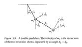
This is from Taylor's classical mechanichs, 11.4, example of finding the Lagrangian of the double pendulum
Relevant figure attached below
Angle between the two velocities of second mass is
$$\phi_2-\phi_1$$
Potential energy
$$U_1=m_1gL_1$$
$$U_2=m_2g[L_1\cos(1-\phi_1)+L_2(1-\phi_2)]$$
$$(U\phi_1,phi_2)=m_1gL_1+m_2g[L_1\cos(1-\phi_1)+L_2(1-\phi_2)]$$
Kinetic energy of the second mass in the double pendulum
$$T_1=\frac{1}{2}m_1L_1^2\dot\phi_1^2$$
$$T_2=\frac{1}{2} m_2[L_1^2\dot\phi_1^2+2L_1L_2\dot\phi_2\dot\phi_1\cos(\phi_1-\phi_2)+L_2^2\dot\phi_2^2]$$
Where $$ T_2=\frac{1}{2}m_2(v_1+L_2\dot\phi_2)^2$$
I am trouble understanding the cos term here. Does it come from the unit vector? Can someone explain why it's involved, because I could not follow why it's here after squaring the velocity for the second kinetic energy
$$2L_1L_2\dot\phi_2\dot\phi_1\cos(\phi_1-\phi_2)$$

 

[PeroK]

If you want to understand where the KE of the second mass comes from, then start with the position of the second mass: $$(x, y) = (L_1\sin \phi_1 +L_2 \sin \phi_2, L_1\cos \phi_1 + L_2\cos \phi_2)$$Then differentiate.

The $\cos(\phi_1 - \phi_2)$ term arises from the relevant trig identity for a cosine of a difference of angles.

 

[P Felds]

Thank you very much

 

[ergospherical]

You get the velocity of the second particle by adding the two contributions $L_1 \dot{\phi}_1$ (varying $\phi_1$ whilst keeping $\phi_2$ fixed) and $L_2 \dot{\phi}_2$ (varying $\phi_2$ whilst keeping $\phi_1$ fixed) vectorially. Joining the vectors tip to tail, the angle between them is $\pi - (\phi_2 - \phi_1)$ so cosine rule states $v^2 = L_1^2 \dot{\phi}_1^2 + L_2^2 \dot{\phi}_2^2 + 2L_1 L_2 \dot{\phi}_1 \dot{\phi}_2 \cos{(\phi_2 - \phi_1)}$.