Modelling of two phase flow in packed bed using conservation equations

Join the discussion
Registration is free. Ask a follow-up in this thread, or start your own.
454 replies · 44K views · last reply
casualguitar said:
I think what's confusing me is that I'm trying to include dm/dt in the ODE solver when I don't need to.

Is this statement correct - we are solving for enthalpy at every point at every time step, and every other parameter is known once enthalpy is known ##(m,T,\rho,Ts,m_j, \dot{m}_{j-1})##

So really the only point of focus is the enthalpy. Once we know the enthalpy everything else is known through the relations you previously developed

Is the above correct?
Yes. Not only that. Maybe now, with the present sweeping tank-at-a-time setup, it might be easier to do the integration ourselves, without using the package ODE integrator. With an implicit integration like backward Euler or Crank-Nicholson, it would only involve solving two linear equations in two unknowns for each sequential tank for each time step. What do you think?
 
Last edited:
Engineering news on Phys.org
Chestermiller said:
Yes. Not only that. Maybe now, with the present sweeping tank-at-a-time setup, it might be easier to do the integration ourselves, without using the package ODE integrator. With an implicit integration like backward Euler or Crank-Nicholson, it would only involve solving two linear equations in two unknowns for each sequential tank for each time step. What do you think?
Hi Chet, just letting you know I am still focusing on the code for this model. I've made some progress and it seems I can do it with the ODE package I previously used. I will continue on with this method for now, as its possible it will be useful in future models
 
  • Like
Likes   Reactions: Chestermiller
Chestermiller said:
Yes. Not only that. Maybe now, with the present sweeping tank-at-a-time setup, it might be easier to do the integration ourselves, without using the package ODE integrator. With an implicit integration like backward Euler or Crank-Nicholson, it would only involve solving two linear equations in two unknowns for each sequential tank for each time step. What do you think?
Looks like there's good news on the model. Finishing up my attempt now. Will get some plots in the next hour or so
 
  • Like
Likes   Reactions: Chestermiller
Chestermiller said:
Yes. Not only that. Maybe now, with the present sweeping tank-at-a-time setup, it might be easier to do the integration ourselves, without using the package ODE integrator. With an implicit integration like backward Euler or Crank-Nicholson, it would only involve solving two linear equations in two unknowns for each sequential tank for each time step. What do you think?
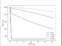
Hi Chet, the code for the model is done I think. I'm setting up various plots now. Temperature distribution for a number of times here:
Line plot of temperature T(K) against position(j) from 0 to 30 at four times: t=0s, t=20s, t=40s and t=60s. Temperature falls from 300 K at position 0; the t=0s curve drops sharply to about 80 K at position 1 and stays flat.

The trend seems to look normal to me i.e. the positions closer to the left increase in temperature first, followed gradually by positions closer to the right
 
Chestermiller said:
Screenshot of Python code using solve_ivp and matplotlib to extract solution arrays and plot T(K) against position(j) at t=0s, 20s, 40s and 60s.
Yes. Not only that. Maybe now, with the present sweeping tank-at-a-time setup, it might be easier to do the integration ourselves, without using the package ODE integrator. With an implicit integration like backward Euler or Crank-Nicholson, it would only involve solving two linear equations in two unknowns for each sequential tank for each time step. What do you think?
And similarly for the fluid enthalpy and mass holdup:
Line plot of enthalpy H (kJ/kg) against position j for four times: t=0s, t=20s, t=40s and t=60s, with the enthalpy curves falling from about 390 kJ/kg at j=0 toward lower values at j=31.

Line plot of mass holdup m (kg) against position j for t=0s, 20s, 40s and 60s: at t=0s the value is 0.25 kg from j=1 onward, while the later curves stay near zero.

The mass holdup plot isn't exactly visually nice to look at. But yes these are the three plots. How does this look to you?

And the code:
Screenshot of Python code defining a two-phase packed bed model: parameters such as Tsat = 105 and volumeV = 0.01/n, plus functions temp(H), mass(H,T) and dpdh(H,T).

Screenshot of Python code in a dark-themed editor defining a function dpdh(H, T) for mass holdup and a function my_system(t, y, n, hIn, Tin, minL, m5, cp5, U, area) for a two-phase model, with starting conditions and time settings.
 
casualguitar said:
And similarly for the fluid enthalpy and mass holdup:
View attachment 293537
View attachment 293538
The mass holdup plot isn't exactly visually nice to look at. But yes these are the three plots. How does this look to you?

And the code:
View attachment 293539
View attachment 293540
This is for 30 tanks, each 1/30 the size of the tank in the single tank model, correct?

In comparison to the single tank model, the time response of this model seems way too fast. The results also seem to show that all the liquid is purged from the bed by 20 sec. This doesn't seem likely. Have you compared the time-dependent results for the first tank in this model with the results of the single tank model for the case of a tank 1/30 the size of the overall bed? The results from this comparison should match.

Also, what does the bed temperature profile look like?
 
Last edited:
Chestermiller said:
In comparison to the single tank model, the time response of this model seems way too fast.
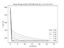
Yes I actually forgot to divide the heat transfer area, and the solid mass by the number of tanks when I was making that graph (see Area and mS parameters are not divided by n). I was looking at the effect of having multiple tanks and forgot to switch back. Heres the fluid temperature plot for n = 32. Note that for the first and last timestep Tf == 0. This is because the numerical derivative dH/dt eliminates two data points. So I've manually added in the IC for the fluid (t=0) again for visual purposes:
Line plot of fluid temperature in Kelvin against position j from 0 to 31 for four times: t=0s flat near 80 K, and t=20s, t=40s and t=60s starting near 300 K and falling along position, ending near 175, 242 and 277 K respectively.


The solid temperature profile:
Line plot of solid temperature T(K) against position(j), with curves for t=0s, 20s, 40s and 60s; the profile flattens and cools toward the far end as time increases.


Comparing this model with the last one now. I don't think they match though, unless I've compared them incorrectly. Checking now

Also, to confirm - if I divide the volume, area and solid mass by n (number of tanks) at the top of the script when declaring variables, then n will not appear at all further down in the computations?
 
Attachments
  • Line plot of fluid temperature in Kelvin against position j from 0 to 31 at t=0s, 20s, 40s and 60s; the curves fall from 300 K at position 0, with the t=0s curve dropping to about 80 K by position 1.
    Screenshot 2021-12-04 at 20.52.39.png
    10.9 KB · Views: 119
Last edited:
Chestermiller said:
Have you compared the time-dependent results for the first tank in this model with the results of the single tank model for the case of a tank 1/30 the size of the overall bed?
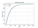
Heres the plot of the fluid temperature for the no spatial dependence model.

Line plot of T_Fluid in kelvin against time from 0 to 30: temperature rises steeply from about 80 K to about 287 K by roughly t = 1, then climbs slowly toward about 300 K by t = 30.


Thinking about this some more, this graph should roughly match the spatial dependence graph at the first position, which it does

To clarify, I divided the volume, area and solid mass by n = 32 in spatial dependence model (I think I actually should have divided by 30 not 32 but anyway). This means that the first tank in the spatial dependence model, and this non-spatial-dependence model are now identical
 
casualguitar said:
Yes I actually forgot to divide the heat transfer area, and the solid mass by the number of tanks when I was making that graph (see Area and mS parameters are not divided by n). I was looking at the effect of having multiple tanks and forgot to switch back. Heres the fluid temperature plot for n = 32. Note that for the first and last timestep Tf == 0. This is because the numerical derivative dH/dt eliminates two data points. So I've manually added in the IC for the fluid (t=0) again for visual purposes:
View attachment 293588

The solid temperature profile:
View attachment 293591

Comparing this model with the last one now. I don't think they match though, unless I've compared them incorrectly. Checking now

Also, to confirm - if I divide the volume, area and solid mass by n (number of tanks) at the top of the script when declaring variables, then n will not appear at all further down in the computations?
These times seem very short compared to what was obtained before by the one tank model of the overall bed. Please prepare a comparison plot of the temperature vs time for the 32nd tank vs the corresponding results from the one tank mode of the overall bed. Please comment on any differences. Thanks.
 
Chestermiller said:
These times seem very short compared to what was obtained before by the one tank model of the overall bed. Please prepare a comparison plot of the temperature vs time for the 32nd tank vs the corresponding results from the one tank mode of the overall bed. Please comment on any differences. Thanks.
Working on the above now

Would it not be the first tank in the 32 tank model that is comparable to the one tank model, as the ICs and BCs would be the same? As the last tank has a variable inlet mass flow which isn't the case in the single tank model
 
casualguitar said:
Working on the above now

Would it not be the first tank in the 32 tank model that is comparable to the one tank model, as the ICs and BCs would be the same? As the last tank has a variable inlet mass flow which isn't the case in the single tank model
No. I want to compare what each of the two models predicts for the temperature as a function of time of the gas coming out of the overall bed.
 
Chestermiller said:
These times seem very short compared to what was obtained before by the one tank model of the overall bed.
The volume/area/solid mass are smaller (32x smaller) compared to the first iteration of the single tank model. The inlet flowrate is the same as before though, so I think it would be expected to have shorter time scales?
Chestermiller said:
Please prepare a comparison plot of the temperature vs time for the 32nd tank vs the corresponding results from the one tank mode of the overall bed. Please comment on any differences. Thanks.
I can't get the single and 32 tank plots on the same plot, so I'll create two. Here is the single tank model plot, where I have taken the volume area and solid mass we had in the original single tank model, and divided them by n = 32:
Line graph titled Single Tank Model plotting Fluid Temperature (K) against time: temperature rises sharply from about 80 K to about 287 K near t = 1, then climbs slowly toward about 299 K by t = 30.

So it takes about 2 seconds before the temperature levels off in the single tank

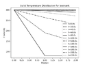
Similarly, for the final tank here is the outlet temperature as a function of time:
Line plot titled 'Fluid Temperature Distribution for last tank': fluid T(K) against time (s), rising from about 80 K to about 290 K over 0 to 80000 s, with a few short vertical spikes near 5000 to 9000 s.

So yes the 32 tank model predicts it will take about 80s for the temperature to level out in the final tank (note the time axis shows x1000 currently. This is 0 to 80s). The single tank model predicts it will take 2 seconds for the temperature in the single tank model to level out.

Also the jumps around the 7 to 10s mark are due to the enthalpy function not being continuous. I'm using the enthalpy derivative to calculate the fluid temperatures

Lastly here's the first tank temperature versus time, showing about 30s to level out (also much slower than the single tank model)
Line plot titled Fluid Temperature Distribution for first tank: fluid T(K) rises from about 80 to near 300 over time 0 to 80000 s, with a dotted curve that levels off near 300 K and several vertical drops in the curve.


Looking into this now

Update: I've got another person to check the newer model and it seems to look ok. Its likely the single tank model that has the error. Checking now
 
Attachments
  • Line plot of fluid temperature T(K) against position j for t=0s to t=5s; the profile drops steeply from 300 K at position 0 to about 80 K and flattens, with curves for later times lying higher.
    Screenshot 2021-12-05 at 15.32.55.png
    12.1 KB · Views: 140
Last edited:
Chestermiller said:
No. I want to compare what each of the two models predicts for the temperature as a function of time of the gas coming out of the overall bed.
Results for this are in post #192. Is it true to say that there is an error in one of the models because the single tank model temperature profile does not match the first tank in the multi-tank model?
ie.
These are not the same:
Line graph titled Single Tank Model plotting Fluid Temperature (K) against time from 0 to 30, showing a blue T_Fluid curve that rises steeply from about 80 K to about 287 K near time 1, then gradually approaches about 299 K.

Line plot titled Fluid Temperature Distribution for first tank, showing fluid T(K) from 0 to about 300 against time (s) from 0 to 80000, a dotted curve rising steeply then levelling off near 300, with a few vertical dotted drops around 5000 and 8500 s.

I haven't seemed to find any errors in either just yet
 
casualguitar said:
Results for this are in post #192. Is it true to say that there is an error in one of the models because the single tank model temperature profile does not match the first tank in the multi-tank model?
ie.
These are not the same:
View attachment 293642
View attachment 293643
I haven't seemed to find any errors in either just yet
The Single tank model for the entire bed should match the 32nd tank of the multi tank model. Well what I really mean is that the time scale should match approximately.
 
Chestermiller said:
The Single tank model for the entire bed should match the 32nd tank of the multi tank model. Well what I really mean is that the time scale should match approximately.
The time scale of the models further back is much closer to the new spatial variation model, which suggests there is some error in the single tank model, which would seem to make sense anyway as the purge time is very low. Looking into it
 
Chestermiller said:
The Single tank model for the entire bed should match the 32nd tank of the multi tank model. Well what I really mean is that the time scale should match approximately.
Getting closer to the solution to this. Its almost definitely got something to do with how I'm adjusting volume, area and solid mass for the single tank model to match the multi tank model values. The reason I think this is because when I fully remove any 'n' from the single tank model i.e. just use the values I used before, the shape of the single and multi tank plots are very similar. Still slightly off in terms of time but they look alike:

Single tank plot:
Line graph titled Single Tank Model plotting Fluid Temperature (K) against time from 0 to 100, legend H_fluid: temperature rises from about -50 K, reaches 0 K near time 20, jumps sharply to about 260 K near time 25, then climbs more gradually to about 380 K at time 100.

Multi tank plot:
Line plot of T(K) against time(s), a dashed black curve labelled none: flat near -50 K until about 3000 s, rising sharply to about 215 K near 4500 s, then climbing more slowly to about 390 K by 80000 s.

So when I try to divide by n it fails and I get a plot similar to the very short time scale in a previous post. So it seems that using volume/n, area/n and solidmass/n is not doing what I expected it to do in the single tank plot

Note the times for the multitask plot are x1000 as I haven't figured out how to scale down the x-axis by 1000. The time range here is 0 to 80s

Do these plots 'match'? Or do you reckon there's an error in one?
 
Edit: The above plots are of time versus enthalpy (forgot to change the y-axis label)

Here are the plots of fluid temperature versus time for both cases:

1) The single tank model:
Line graph titled Single Tank Model plotting Fluid Temperature (K) against time. Temperature rises slowly from about 80 K to about 105 K by time 20, holds near 105 K until about 24, then jumps sharply to about 165 K and keeps rising, reaching about 285 K at time 100.

Last tank in the 32 tank model (where actual t = t/1000):
Line plot titled Fluid Temperature Distribution for last tank, showing T Fluid (K) from about 80 to 290 against time from 0 to 80000. The curve stays near 80 K, rises sharply around time 5000, then climbs and flattens toward about 290 K by time 80000. Two short vertical dashed spikes appear near time 5000 and 8000.

These plots seem to show a similar trend and an approximately equal 'levelling off' time for the fluid temperature. The fix (if you agree these plots look ok) was in how I was dividing up the volume, area, and solid mass per unit area

I am absolutely ready to work some more on this model today if you think we're ready to do some more
 
Last edited:
casualguitar said:
Getting closer to the solution to this. Its almost definitely got something to do with how I'm adjusting volume, area and solid mass for the single tank model to match the multi tank model values. The reason I think this is because when I fully remove any 'n' from the single tank model i.e. just use the values I used before, the shape of the single and multi tank plots are very similar. Still slightly off in terms of time but they look alike:

Single tank plot:
View attachment 293646
Multi tank plot:
View attachment 293648
So when I try to divide by n it fails and I get a plot similar to the very short time scale in a previous post. So it seems that using volume/n, area/n and solidmass/n is not doing what I expected it to do in the single tank plot

Note the times for the multitask plot are x1000 as I haven't figured out how to scale down the x-axis by 1000. The time range here is 0 to 80s

Do these plots 'match'? Or do you reckon there's an error in one?
They have to approximately match on the time scale. The multi-tank time variation of the temperature leaving the tank should be sharper (closer to a square wave) than the single tank model of the overall bed. But they need to be close to one another. The multi-tank should have lower temperatures at short times and higher temperatures at longer times; so they have to cross over one another.

The time scale for the response should be roughly on the order of $$\frac{m_SC_S}{UA}$$What value do you calculate for this?

I'm going to try to leave the coding up to you and only offer guidance on model structure.
 
Chestermiller said:
The time scale for the response should be roughly on the order of mSCSUAWhat value do you calculate for this?
11 for this (##mS = 1, C_ps = 1.1, U = 1, A = 0.1##). Is this time scale term an approximation for the time it should take to reach steady state in a tank?
Chestermiller said:
The multi-tank time variation of the temperature leaving the tank should be sharper (closer to a square wave) than the single tank model of the overall bed.
Ok so are you saying there is an error in the multi-tank model because it doesn't really cross over the single tank model at all? i.e. higher temperature at low and high times

Chestermiller said:
I'm going to try to leave the coding up to you and only offer guidance on model structure.
Thats good with me, I don't think the code will get much more complex math-wise than it is currently anyway
 
casualguitar said:
11 for this (##mS = 1, C_ps = 1.1, U = 1, A = 0.1##). Is this time scale term an approximation for the time it should take to reach steady state in a tank?
For the bed
casualguitar said:
Ok so are you saying there is an error in the multi-tank model because it doesn't really cross over the single tank model at all? i.e. higher temperature at low and high times
I don’t know which model has the error (or errors). This is part of doing the validation of the model.
 
Chestermiller said:
For the bed

I don’t know which model has the error (or errors). This is part of doing the validation of the model.
Got it my bad working on this now.

One approach to do this could be to reduce to 3 tanks and do some manual calculations to see which model values don't match the manually calculated versions. Trying this now
 
  • Like
Likes   Reactions: Chestermiller
Chestermiller said:
What were the units of that approximate time scale calculation?
##\frac{kg*\frac{kJ}{kgK}}{\frac{W}{m2K}*m2}## = ##\frac{kJ}{W}## = ##1000*s## == kilo seconds I suppose?

Changing the heat capacity units to ##\frac{J}{kgK}## gives a value of 11,000s for the time scale of the response
 
casualguitar said:
##\frac{kg*\frac{kJ}{kgK}}{\frac{W}{m2K}*m2}## = ##\frac{kJ}{W}## = ##1000*s## == kilo seconds I suppose?

Changing the heat capacity units to ##\frac{J}{kgK}## gives a value of 11,000s for the time scale of the response
You got to be kidding. Changing the units of heat capacity doesn’t change the value of this quantity. The result is still 1100 sec.
 
Chestermiller said:
You got to be kidding. Changing the units of heat capacity doesn’t change the value of this quantity. The result is still 1100 sec.
Ah no I agree it doesn't change the value, just the unit of time i.e. from kilo seconds to seconds. My original value of 11 was in kilo seconds (according to the above). Multiplying by 1000 to convert to seconds. Is this incorrect?

Apologies for the confusion here. I think it might be best for me to spend some time looking at the output of the spatial variation model (and doing some manual calculations to check the model output). Otherwise I'm wasting your time and mine
 
Chestermiller said:
1100 is correct
So 1100s is the approx time it would take for the solid temperature to reach steady state i.e. the timescale. The solid temperature will converge exponentially towards 300 but will never reach 300. Where would the cut-off point be here? Say within 0.1K or so? I can check the exact time required for the cutoff to be reached.
 
Attachments
  • Line plot titled Solid Temperature Distribution for last tank, showing T Solid (K) from about 80 to 300 against Position from 0.00 to 2.00 for eleven times from t=0.0s to t=220.0s, with a legend listing each time.
    Screenshot 2021-12-06 at 22.13.20.png
    19.2 KB · Views: 127
casualguitar said:
So 1100s is the approx time it would take for the solid temperature to reach steady state i.e. the timescale. The solid temperature will converge exponentially towards 300 but will never reach 300. Where would the cut-off point be here? Say within 0.1K or so? I can check the exact time required for the cutoff to be reached.
We have got to take a step back, and make sure that the single tank model of the entire bed is getting the right answer. This can be checked by running a calculation in which the model can be solved analytically. Such a case would be if the stream entering the tank is a liquid at a temperature below the saturation temperature, and the bed is initially at a colder temperature. Then we can compare the analytic solution to the time-dependent numerical solution to make sure that the time scale we get numerically is correct.

After that, I have developed an even simpler version of the multi-tank model that is easier to implement, and less prone to coding error. I have shown that the multi-tank model is equivalent to n tanks in series identical in every respect to that being used in the single tank model of the entire bed, but with a mass flow to the first tank in the series equal to n times the actual mass flow rate to the actual bed. I will document the new development once we have validated the single tank model.
 
Chestermiller said:
We have got to take a step back, and make sure that the single tank model of the entire bed is getting the right answer. This can be checked by running a calculation in which the model can be solved analytically. Such a case would be if the stream entering the tank is a liquid at a temperature below the saturation temperature, and the bed is initially at a colder temperature. Then we can compare the analytic solution to the time-dependent numerical solution to make sure that the time scale we get numerically is correct.
Great! I follow the first paragraph idea. So focusing on the first paragraph - we will have ## h<=0## at all times, meaning we can use the liquid correlations for temperature and mass holdup i.e. ##T = T_{SAT} + \frac{h}{C_{PL}}## and ##m = \rho_{L}*V##.

Letting Tsat = 105, Tin = 90, and T0 = 80 (bed/fluid initial temperature), for the single tank model, this is the plot for the liquid phase only model:
Line plot titled Single Tank Model - Liquid Phase Only: temperature in K versus time, with T_Fluid (blue) and T_solid (green) rising from 80 K to about 90 K and levelling off near 1200.

If we are expecting a timescale of 1100s here this seems to line up relatively ok.

I did the same for gas phase only - where Tsat = 105, Tin = 300 and T0 = 200 (bed/fluid initial temperature), for the single tank model. Gas phase plot looks like this:
Line graph titled Single Tank Model - Gas Phase Only, plotting Temperature (K) against time from 0 to 300. Blue T_Fluid curve jumps from 200 to about 234 K, then rises to 300 K. Green T_solid curve starts at 200 K and rises gradually to 300 K.

Seems to look off, due to that fluid temperature jump at the start. Will do some diagnostic testing on the gas phase section
 
Attachments
  • Line plot titled Single Tank Model of temperature in kelvin against time from 0 to 1200, with T_Fluid (blue) and T_solid (green) rising from 80 K to about 90 K and levelling off.
    Screenshot 2021-12-07 at 13.18.02.png
    14.5 KB · Views: 120
casualguitar said:
Great! I follow the first paragraph idea. So focusing on the first paragraph - we will have ## h<=0## at all times, meaning we can use the liquid correlations for temperature and mass holdup i.e. ##T = T_{SAT} + \frac{h}{C_{PL}}## and ##m = \rho_{L}*V##.

Letting Tsat = 105, Tin = 90, and T0 = 80 (bed/fluid initial temperature), for the single tank model, this is the plot for the liquid phase only model:View attachment 293726
If we are expecting a timescale of 1100s here this seems to line up relatively ok.

I did the same for gas phase only - where Tsat = 105, Tin = 300 and T0 = 200 (bed/fluid initial temperature), for the single tank model. Gas phase plot looks like this:
View attachment 293728
Seems to look off, due to that fluid temperature jump at the start. Will do some diagnostic testing on the gas phase section
Do you know how to solve this analytically (two linear coupled ODEs in two unknowns)?