Chestermiller said:
How about next doing the liquid-only calculation with many more tanks
Got caught up with some report writing this evening. Back in action now
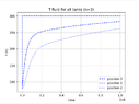
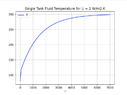
Heres the liquid-only plot with more tanks (n=32). Plotting the temperature profile for the first and last tank here:
I checked this against the single tank plot for a 32x flowrate and they do match
Chestermiller said:
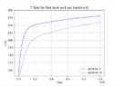
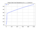
and doing the 3 tank version with the full temperature range with inlet at 300 K
I was about to post and noticed this plot was incorrect. I took out some gas functionality to simplify the code so I could spot the error. Its a quick job to put this back in so I'll do this first thing tomorrow
Chestermiller said:
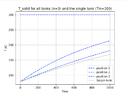
Now how about plotting the temperature vs time for all three tanks, and also showing on the same plot the result from the single tank model for the overall bed.
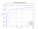
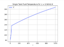
Looking into a good way to do this overlay plot still. For now here it is as two separate plots:
Temperature vs time for all three tanks (liquid phase only):
So now we seem to have a working model for a single and multi-tank setup. I can think roughly about what the future models would hopefully look like, however to get there, what do you think are the next best steps?
So some simplifications we've made:
- The enthalpy/mass holdup relations. In previous posts you mentioned we would stick to correlations like these. If its an option then we can also use H(T,P) methods already made in other Python libraries i.e. just use a property calculation library to calculate enthalpy
- The heat of vaporisation. Right now we're leaving this as a constant. I have methods again from thermo libraries that treat this as a function of temperatures so we have the option to use this
- The saturation conditions. Right now we've got Tsat defined at the top as a constant. I have Tsat(P) functionality so I could use this no bother to get the saturation temperature
- The quality. Right now we get around the quality with the saturation zone relations
- The fluid. So assuming a pure fluid let's us have one saturation temperature. Air is a mixture so we'll have a bubble/dew point. This definitely sounds difficult to implement. That said I have a lot of useful functionality from the thermo property libraries like dew/bubble point temperature calculations for mixtures, Pressure-Enthalpy flash functionality, really anything we would need. So the important bit here is the actual algorithm, the functionality is available
- Lastly obviously we have constant heat capacity, etc. This can easily be switched out for temperature/pressure dependent values later on but yes its probably best to leave them as constant for now to avoid cluttering etc
- The U value. I've put a value of 1 (out of thin air). We could improve on that
From the above it seems that it might be best to stick with a pure fluid until we get to a late stage model, and then switch to a mixture. Developing the pure fluid model to late-stage would also give us the ability to test pure fluids in the packed bed
So yes, in terms of the next step or two, what do you think is best?