Understanding Theorem 3.4: Mean Value Theorem & Cauchy Riemann Equations

[Math Amateur]

I am reading "Complex Analysis for Mathematics and Engineering" by John H. Mathews and Russel W. Howell (M&H) [Fifth Edition] ... ...

I am focused on Section 3.2 The Cauchy Riemann Equations ...

I need help in fully understanding the Proof of Theorem 3.4 ...The start of Theorem 3.4 and its proof reads as follows:View attachment 9350In the above proof by Mathews and Howell we read the following:

" ... ... The partial derivatives \(\displaystyle u_x\) and \(\displaystyle u_y\) exist, so the mean value theorem for real functions of two variables implies that a value \(\displaystyle x*\) exists between \(\displaystyle x_0\) and \(\displaystyle x_0 + \Delta x\) such that we can write the first term in brackets on the right side of equation (3-17) as

\(\displaystyle u(x_0 + \Delta x, y_0 + \Delta y) - u(x_0, y_0 + \Delta y) = u_x(x*, y_0 + \Delta y) \Delta x \) ... ... "

Can someone please explain how exactly the mean value theorem for real functions of two variables implies that a value \(\displaystyle x*\) exists between \(\displaystyle x_0\) and \(\displaystyle x_0 + \Delta x\) such that we can write the first term in brackets on the right side of equation (3-17) as

\(\displaystyle u(x_0 + \Delta x, y_0 + \Delta y) - u(x_0, y_0 + \Delta y) = u_x(x*, y_0 + \Delta y) \Delta x\) ... ...
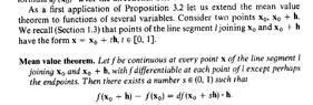
Peter[ NOTE ... ... In Wendell Fleming's book: "Functions of Several Variables" (Second Edition) the Mean Value Theorem reads as follows:View attachment 9351... ... ]

 

[Jhoneine]

The Mean Value Theorem for real functions of two variables states that if a function f(x,y) is continuous on some rectangle R and differentiable on the interior of R then there exists some point (x*,y*) in the interior of R such that f(x_2,y_2)-f(x_1,y_2) =f_x(x*,y_2)(x_2-x_1)andf(x_2,y_2)-f(x_2,y_1)=f_y(x_2,y*)(y_2-y_1). In our case, we are dealing with a function u(x,y) which is assumed to be differentiable on some region. Applying the Mean Value Theorem to this function, we see that there exists some point (x*,y_0+\Delta y) in the interior of the region such that u(x_0 + \Delta x, y_0 + \Delta y) - u(x_0, y_0 + \Delta y) = u_x(x*, y_0 + \Delta y) \Delta x. We can see from this that x* must lie between x_0 and x_0+\Delta x, since otherwise the right side of the equation would not be equal to the left side.

 

[soloenergy]

Hi Peter,

The mean value theorem for real functions of two variables states that if a function f(x,y) is continuous on a closed and bounded region R and has continuous partial derivatives u_x and u_y at every point in R, then there exists a point (x*, y*) in R such that:

f(x_2,y_2) - f(x_1,y_1) = u_x(x*, y*) (x_2 - x_1) + u_y(x*, y*) (y_2 - y_1)

In this case, the function u(x,y) is continuous on the closed and bounded region R = [x_0, x_0 + \Delta x] x [y_0, y_0 + \Delta y] and has continuous partial derivatives u_x and u_y at every point in R. Therefore, the mean value theorem can be applied to the first term in brackets on the right side of equation (3-17) to obtain:

u(x_0 + \Delta x, y_0 + \Delta y) - u(x_0, y_0 + \Delta y) = u_x(x*, y_0 + \Delta y) \Delta x

where (x*, y_0 + \Delta y) is a point in the region R = [x_0, x_0 + \Delta x] x [y_0, y_0 + \Delta y]. This is because the mean value theorem guarantees the existence of such a point x* between x_0 and x_0 + \Delta x, and since u_x is continuous, it can be evaluated at this point.

I hope this helps clarify the proof for you. Let me know if you have any other questions. Happy studying!