Why is my simulation of projectile trajectory with air resistance wrong?

In summary, the conversation discusses a simulation created in Python to determine the ideal angle for throwing a stone in a lake with air resistance. The simulated trajectory was found to be wrong and the participants discussed the expected concave shape of the trajectory. However, there was a coding error that caused the trajectory to bend upwards. The correct method for determining velocity was discussed and the issue was resolved.
  • #1
fisicist
46
7
Hey!

This started very harmless... A friend and I were throwing stones in a lake. Mine didn't get very far, he was teasing me "What was the ideal angle again?". Of course, I know it should be 45°. I replied in jest: "That's because I'm considering air resistance!" Then we had a discussion what the ideal angle should be with air resistance considered.
So I wrote a simulation in Python. It was just for fun... But I encountered an issue that I don't quite understand: The simulated trajectory is wrong. I hope someone can help me understand where this is coming from, and perhaps give me some hint how to fix it.

My code is:
Python:
import numpy as np
import matplotlib.pyplot as plt
from scipy.integrate import solve_ivp

c = 7
v = 5

# f gives phase space velocity
# z = [x, y, v_x, v_y]
# f(t, z) = [v_x, v_y, a_x, a_y]
def f(t, z):
    global c
    vel = z[2:]
    friction = -c * np.absolute(vel) * vel
    gravity = [0, -0.5]
    accel = friction + gravity
    return np.concatenate((vel, accel))

def hit_ground(t, z): return z[1]
hit_ground.terminal = True
hit_ground.direction = -1

t_eval = np.linspace(0, 100, 10000)

def v_init(theta):
    global v
    return v * np.array([np.cos(theta), np.sin(theta)])

thetas = np.linspace(0.0, np.pi/2, 181)
dists = np.array([])
plt.subplot('211')
for counter,theta in enumerate(thetas):
    init = np.concatenate((np.array([0., 0.]), v_init(theta)))
    sol = solve_ivp(f, [0, 100], init, t_eval = t_eval, events=hit_ground)
    if counter % 40 == 0:
        plt.plot(sol.y[0,:], sol.y[1,:], label='{:4.0f} °'.format(theta*180/np.pi))
        plt.gca().quiver(sol.y[0,::70], sol.y[1,::70], 1000*sol.y[2,::70], 1000*sol.y[3,::70])
    dists = np.append(dists, [sol.y[0,-1]])
#plt.gca().set_aspect('equal', adjustable='box')
plt.legend(loc='upper left')
plt.xlabel('$x$')
plt.ylabel('$y$')

plt.subplot('212')
plt.plot(thetas*180/np.pi, dists, 'r-')
best_angle = thetas[np.argmax(dists)]
plt.gca().axvline(x = best_angle*180/ np.pi)
print('{:3.1f}'.format(best_angle*180/ np.pi))
plt.xlabel('angle [°]')
plt.ylabel('distance')

plt.show()

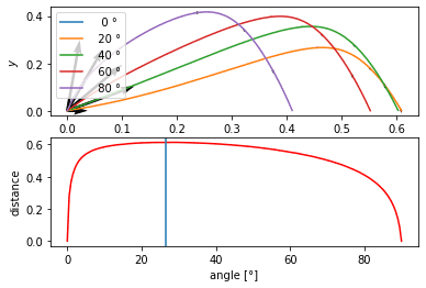
Result:
angles.png


This shouldn't happen... As you can see, the curves bend upward, i.e. are not concave. Even without knowing the exact solution [itex]y(x)[/itex], it is easy to prove it should be a concave function.
The model is [itex]\ddot{x} = - c \dot{x}\sqrt{\dot{x}^2+\dot{y}^2}, \ddot{y} = - c \dot{y} \sqrt{\dot{x}^2+\dot{y}^2} - \frac 1 2 [/itex]
By the chain rule, [itex]\frac{d^2 y}{d^2 x} (x(t)) = \frac{\ddot{y}}{\dot{x}^2} - \dot{y}\frac{\ddot{x}}{\dot{x}^3} = \frac{1}{\dot{x}^2} \left( -2 c \dot y \sqrt{\dot{x}^2+\dot{y}^2} - \frac 1 2 \right)[/itex]
Therefore, at least as long as [itex]\dot{y} \geq 0[/itex], this should be a concave function. If I through it downwards with high speed, it might get convex there, but not as long as the motion is upward.

CORRECTION: By the chain rule: [itex]\frac{d^2 y}{d^2 x} (x(t)) = -\frac{1}{2 \dot{x}^2} \leq 0[/itex]

So, what is wrong with the simulation? I know the time subdivision is not very high. But that shouldn't matter, because also in the discretized model, the velocity vector should be shortened and then get a downward contribution in every step. That's not what I see in the plot.

Any ideas, anyone?
 
Last edited:
Physics news on Phys.org
  • #2
fisicist said:
Therefore, at least as long as [itex]\dot{y} \geq 0[/itex], this should be a concave function.
Hmm, I am not seeing that, where do you get that condition from?
 
  • #3
Dale said:
Hmm, I am not seeing that, where do you get that condition from?
[itex]1/\dot{x}^2 \geq 0[/itex] manifestly, so it remains to check that [itex]-2 c \dot{y} \sqrt{\dot{x}^2+\dot{y}^2}-\frac 1 2 \leq 0 [/itex] in order for [itex]d^2 y/ d x^2 \leq 0[/itex] (i.e. concavity). But [itex]-2 c \sqrt{\dot{x}^2 +\dot{y}^2}[/itex] is always negative, so if [itex]\dot{y} \geq 0[/itex], everything is negative.
 
  • #5
Dale said:
Hmm, I am not seeing that, where do you get that condition from?
An informal argument for concavity: The drag is always tangential so it doesn't change the direction, while gravity is always bending the path down.

Looks like some lift sneaked in somewhere.
 
Last edited:
  • #6
Hey sorry, I've made a sign error. The two friction terms compensate each other, not add up. Actually not surprising: Without gravity, motion is along a straight line.
I will correct it. Correct is
[itex] d^2 y / dx^2 = - \frac{1}{2 \dot{x}^2} [/itex]
Still, it's concave. In fact, it is *always* concave, even if I throw the stone downwards.
 
  • #7
fisicist said:
As you can see, the curves bend upward, i.e. are not concave.
I would call bending upward and then downward "concave". Bending only downward would be "convex", and what you would expect here.

Have you tried coding a simple Euler integration yourself?
 
  • #8
A.T. said:
I would call bending upward and then downward "concave". Bending only downward would be "convex", and what you would expect here.

Have you tried coding a simple Euler integration yourself?

The standard definition used in mathematics (in fields such as calculus of variations, 'convex analysis' or 'convex optimization') is that a function is convex if its epigraph [itex]\operatorname{epi}f := \lbrace (x, y) : y \geq f(x) \rbrace[/itex] is a convex set. For a twice differentiable function, this is equivalent to [itex]f'' \geq 0[/itex]. A function [itex]f[/itex] is concave if [itex]-f[/itex] is convex.
 
  • #9
fisicist said:
The standard definition used in mathematics (in fields such as calculus of variations, 'convex analysis' or 'convex optimization') is that a function is convex if its epigraph [itex]\operatorname{epi}f := \lbrace (x, y) : y \geq f(x) \rbrace[/itex] is a convex set. For a twice differentiable function, this is equivalent to [itex]f'' \geq 0[/itex]. A function [itex]f[/itex] is concave if [itex]-f[/itex] is convex.
Ok, thanks. I would suggest coding a simple Euler integration. It should never bend upwards.
 
  • #10
Thank you to everyone who replied here!
I found the error. It's not a mathematical or numerical curiosity, but a simple coding error. Namely,
Python:
np.absolute(vel)
does not give [itex]\vert \dot{\mathbf x} = \sqrt{\dot{x}^2+\dot{y}^2}[/itex], as I thought it would, but [itex](\vert \dot x \vert, \vert \dot y \vert )^T[/itex], and
Python:
np.absolute(vel) * vel
does not give [itex]\dot{\mathbf{x}} \vert \dot{\mathbf{x}} \vert[/itex], as I thought it would, but [itex](\dot{x} \vert \dot{x} \vert, \dot{y} \vert \dot{y} \vert )^T[/itex].

The correct way to do it is
Python:
np.sqrt(vel.dot(vel)) * vel
 
  • Like
  • Informative
Likes jim mcnamara and Dale
  • #11
fisicist said:
Thank you to everyone who replied here!
I found the error. It's not a mathematical or numerical curiosity, but a simple coding error. Namely,
Python:
np.absolute(vel)
does not give [itex]\vert \dot{\mathbf x} = \sqrt{\dot{x}^2+\dot{y}^2}[/itex], as I thought it would, but [itex](\vert \dot x \vert, \vert \dot y \vert )^T[/itex], and
Python:
np.absolute(vel) * vel
does not give [itex]\dot{\mathbf{x}} \vert \dot{\mathbf{x}} \vert[/itex], as I thought it would, but [itex](\dot{x} \vert \dot{x} \vert, \dot{y} \vert \dot{y} \vert )^T[/itex].

The correct way to do it is
Python:
np.sqrt(vel.dot(vel)) * vel

Congratulation! So what is the ideal angle when you include air resistance?
 
  • #12
For anyone interested in the physics: Qualitatively, the result is similar.
angles-corr.png

Qualitatively, the best angle decreases rapidly the higher the friction is:
bestangles.png
 
  • Like
Likes William Crawford
  • #13
Run your sim on a baseball and see if 40 deg gives the maximum range.
 
  • #14
fisicist said:
The correct way to do it is
Python:
np.sqrt(vel.dot(vel)) * vel
Or:
Python:
np.linalg.norm(vel) * vel
https://docs.scipy.org/doc/numpy/reference/generated/numpy.linalg.norm.html
fisicist said:
For anyone interested in the physics: Qualitatively, the result is similar.
View attachment 247485
Qualitatively, the best angle decreases rapidly the higher the friction is:
View attachment 247487
Regarding your stone throwing contest:

You could plot the optimal angle as function of the object's density for a given realistic object shape/size and throw speed. It could be that for stones the angle is pretty close to 45° at the speed you can throw, while for light balls (like tennis) it makes sense to aim lower.

Bio-mechanics complicates matters because you won't achieve the same throw speeds for any angle.

Finally, your friend might simply throw much faster, and thus further, even at sub optimal angles.
 
Last edited:

1. Why does my simulation of projectile trajectory with air resistance not match my calculations?

There could be several reasons for this discrepancy. One possibility is that your simulation is not taking into account all the relevant factors, such as wind speed and direction, or the shape and size of the projectile. Another possibility is that there are errors in your calculations or in the parameters you have entered into the simulation. It is important to carefully review your inputs and make sure they are accurate.

2. How can I improve the accuracy of my simulation of projectile trajectory with air resistance?

To improve the accuracy of your simulation, you can try adjusting the parameters to better match the real-world conditions. This could include using more precise measurements for variables like air density and drag coefficient, or incorporating more complex equations to account for factors like spin and turbulence. It may also be helpful to compare your simulation results to real-world data or other reliable sources to identify areas for improvement.

3. Does air resistance affect the trajectory of a projectile more at higher or lower velocities?

Air resistance has a greater impact on the trajectory of a projectile at higher velocities. This is because as the speed of the projectile increases, the force of air resistance also increases, making it more difficult for the projectile to maintain its initial velocity and trajectory. This is why projectiles with lower velocities, such as arrows or bullets, are less affected by air resistance compared to faster-moving objects like rockets or airplanes.

4. How does the angle of launch affect the trajectory of a projectile with air resistance?

The angle of launch can greatly affect the trajectory of a projectile with air resistance. In general, a higher launch angle will result in a longer flight time and a shorter horizontal distance traveled, while a lower launch angle will result in a shorter flight time and a longer horizontal distance. This is because a higher angle allows the projectile to spend more time in the air, while a lower angle results in a more direct path towards the target.

5. Can I completely eliminate the effects of air resistance in my simulation of projectile trajectory?

No, it is not possible to completely eliminate the effects of air resistance in a simulation of projectile trajectory. Air resistance is a natural force that will always have some impact on the motion of an object. However, you can minimize its effects by using accurate and precise parameters, as well as more advanced equations that take into account additional factors like air density and turbulence. Keep in mind that even with these adjustments, there will still be some degree of error in the simulation due to the unpredictable nature of air resistance.

Similar threads

Replies
7
Views
6K
  • Introductory Physics Homework Help
Replies
3
Views
734
  • Electromagnetism
Replies
8
Views
1K
  • Advanced Physics Homework Help
Replies
6
Views
1K
  • Calculus and Beyond Homework Help
Replies
7
Views
2K
  • Advanced Physics Homework Help
Replies
7
Views
1K
  • Differential Equations
Replies
8
Views
1K
  • General Math
Replies
4
Views
7K
  • Advanced Physics Homework Help
Replies
2
Views
2K
  • Programming and Computer Science
Replies
2
Views
16K
Back
Top