Apostol Problem on ODE applied to Population Growth

[zenterix]

Homework Statement

The following two problems are from chapter 8.7 "Introduction to Differential Equations" of Apostol's Calculus Volume I.

Problem 13. (Prelude to Problem 14, about which my question is)

Express $x$ as a function of $t$ for the growth law

$$\frac{dx}{dt}=kx(M-x)$$

with $k$ and $M$ both constant. Show that

$$x(t)=\frac{M}{1+e^{-kM(t-t_1)}}\tag{8.23}$$

where $t_1$ is the time at which $x=M/2$.

Problem 14.

Assume the growth law in formula 8.23 of exercise 13, and suppose a census is taken at three equally spaced times $t_1,t_2,t_3$, the resulting numbers being $x_1,x_2,x_3$. Show that this suffices to determine $M$ and that, in fact, we have

$$M=x_2\frac{x_3(x_2-x_1)-x_1(x_3-x_2)}{x_2^2-x_1x_3}\tag{8.24}$$

Relevant Equations

My question is strictly about exercise 14.

Exercise 13 is a relatively simple matter (and I include at the end my solution to it).

First of all, a few observations

1) It is not clear if the $t_1$ used in problem 14 is the same $t_1$ from problem 13 where $x(t_1)=\frac{M}{2}$.

However, if it were, then the problem seems like it wouldn't make too much sense because we'd have $M=2x_1$ and that'd be it (though this wouldn't match the expression the problem has for $M$).

We would be able to solve for $k$ as well in this case with just one census reading.

2) From (8.23) it seems that the population never actually reaches $M$. It just gets really close from below.

Now let me rewrite the equation for $x$ as follows

$$x(t)=\frac{M}{1+e^{-kM(t-t_h)}}$$

where now $t_h$ is such that $x(t_h)=\frac{M}{2}$.

I've tried a few things but am a bit stuck.

Each attempt is a lot to type so I will have to screenshot them.

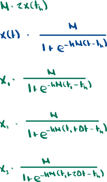
First I tried to just plug the values in

But this doesn't seem to tell me much.

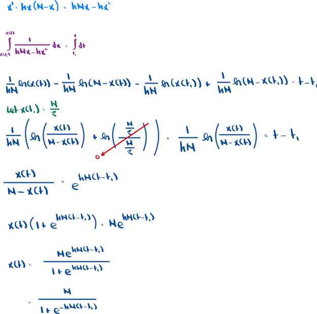
Well, I will post now, as I continue to think about this problem.Since it will be too much work to write out all my work for problem 13 in equations, here is a screenshot of the work

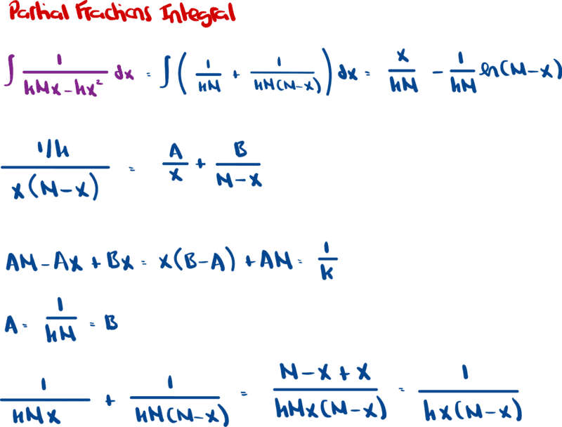
Note that I used partial fractions to solve the integral in purple, and the calculations were as follows

 

[pasmith]

First of all, a few observations

1) It is not clear if the $t_1$ used in problem 14 is the same $t_1$ from problem 13 where $x(t_1)=\frac{M}{2}$.

It isn't, for the following reason:

However, if it were, then the problem seems like it wouldn't make too much sense because we'd have $M=2x_1$ and that'd be it (though this wouldn't match the expression the problem has for $M$).

We would be able to solve for $k$ as well in this case with just one census reading.

2) From (8.23) it seems that the population never actually reaches $M$. It just gets really close from below.

Now let me rewrite the equation for $x$ as follows

$$x(t)=\frac{M}{1+e^{-kM(t-t_h)}}$$

where now $t_h$ is such that $x(t_h)=\frac{M}{2}$.

I've tried a few things but am a bit stuck.

The key is that the times are equally spaced, so $t_2 = t_1 + T$, $t_3 = t_1 + 2T$. Then you have $$\begin{split} x_1 &= \frac{M}{1 + A} \\ x_2 &= \frac{M}{1 + e^{-kM(t_1 + T - t_h)}} = \frac{M}{1 + AB} \\ x_3 &= \frac{M}{1 + e^{-kM(t_1 + 2T - t_h)}} = \frac{M}{1 + AB^2} \end{split}$$ where $A = e^{-kM(t_1 - t_h)}$ and $B = e^{-kMT}$. Here I think the strategy is to find an expression for $B$ from the second equation, and set the square of that equal to the expression for $B^2$ obtained from the third equation; then the first equation can be used to eliminate $A$.