Discussion Overview
The discussion revolves around calculating the magnetic field strength of a cylindrical magnet and its implications for determining magnetic flux through a wire loop. Participants explore theoretical approaches, mathematical formulations, and practical considerations, including the use of simulations.
Discussion Character
- Exploratory
- Technical explanation
- Mathematical reasoning
- Debate/contested
Main Points Raised
- One participant presents the equation for magnetic flux and expresses uncertainty about calculating the magnetic field strength (B) of a cylindrical magnet, suggesting the potential use of the Biot-Savart law.
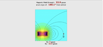
- Another participant notes that calculating the magnetic field strength is generally challenging and often requires simulations, referencing an external link that provides approximations.
- A participant asks for clarification on determining the distance representing the air gap between testing points in the context of the magnetic field strength calculation.
- Several participants discuss two general approaches to magnetostatics, focusing on the use of scalar and vector potentials in the context of a hard ferromagnet, referencing macroscopic Maxwell equations and constitutive relations.
- Participants provide detailed mathematical formulations related to the scalar potential for H and the vector potential for B, discussing the implications of magnetization and current density.
- One participant expresses gratitude for the detailed contributions, indicating that the information is helpful.
Areas of Agreement / Disagreement
There is no consensus on a definitive method for calculating the magnetic field strength, with multiple approaches and models being discussed. Participants express varying levels of confidence in the methods proposed, and the discussion remains unresolved.
Contextual Notes
The discussion includes complex mathematical formulations and assumptions related to magnetostatics, which may not be universally applicable. The dependence on specific conditions, such as the type of magnet and the presence of free currents, is noted but not resolved.