I Confusion in variation derivative

[weezy]

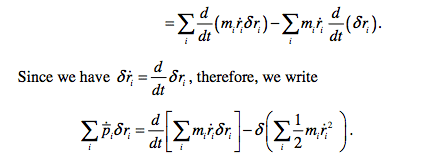
This link shows us how to derive Hamilton's generalised principle starting from D'Alembert's principle. While I had no trouble understanding the derivation I am stuck on this particular step.

I can't justify why $\frac{d}{dt} \delta r_i = \delta [\frac{d}{dt}r_i]$. This is because if I consider $\delta \dot r_i$ to be spatial variation in velocity of a particle as I shift my origin keeping time constant, doesn't it stay the same i.e. doesn't $\delta \dot r_i = 0$?

Also if I assume that throughout a large section of the path $\delta r_i = Constant$ don't I get $\frac{d}{dt} \delta r_i = 0 ?$

Is this supposed to have a non-zero value or are we simply playing with 0's here?

Edit : If I assume $\delta$ to act like an operator on $r$ I don't see a problem arising as we've done in Quantum mechanics for commuting operators by interchanging their order. Can we say the same for this?

 

[jambaugh]

This is technically an assumed constraint and not a derived result. But it follows from the understanding of what the functional differential is doing.
You are introducing a variation in the time dependent variable: r_i \to \tilde{r}_i = r_i + \delta r_i. We understand that we are to extend the time derivative without introducing additional independent variations so that \dot{r}_i \to \tilde{\dot{r}}_i = \dot{\tilde{r}_i}. It is implied that the functional variation behaves just like a standard differential in that it is a local linear deviation from the previous value.

The action here of \delta on r is the same as the action of d on an independent vector variable. If you had a function of a vector: f(\mathbf{x}) then its variation is
df(\mathbf{x}) = \lim_{h\to 0}\frac{ f(\mathbf{x} + h \mathbf{dx})-f(\mathbf{x})}{h} = \frac{df}{d\mathbf{x}}[\mathbf{dx}]

Here the total derivative\frac{df}{\mathbf{dx}} of f is a linear mapping from the differential vector \mathbf{dx} to the range of f. The differential \mathbf{dx}=\langle dx_1, dx_2,dx_3\cdots\rangle is an independent auxiliary (vector) variable representing a local linear coordinate with origin at the point indicated by the original vector \mathbf{x}. You can say that the differential operator d maps the original independent vector variable to this auxiliary variable but keep in mind that it is an independent variation. While we are at it you can think of the vector as a function from its component index into the reals. x(1) = x_1, x(2)=x_2, etc. The non-trivial action of the differential is effected by its action on functions of \mathbf{x}.

Now consider a continuously indexed "vector" i.e. a continuous function r(t) thinking of t as the index. To avoid confusing the same kind of differential of a function, i.e. dr(t) = \dot{r}(t)dt we use the different differential notation: \delta r to indicate (in the function space where r lives) an independent variation of the choice of function r(t) \to r(t) + \delta r(t).

The fact that the derivative of the variation is the variation of the derivative is no more mysterious than the fact that for the \mathbf{x} example the variation in the difference of successive components is the difference in the variation of successive components:
\Delta: \mathbf{x} \mapsto x_2 - x_1
and thus
d\Delta \mathbf{x} = \Delta d\mathbf{x} = dx_2 - dx_1

But the short answer is that the "justification" comes down to the fact that the derivative of a sum is the sum of the derivatives and we are (independently) varying the function additively: r\mapsto r+ \delta r.