Difference equation tutorial: draft of part I

[chisigma]

Dear friends of MHB
some months ago I wrote for MHF a tutorial on the Difference equations and the reason of that was the difficulties I noticed in the treatment of difference equations, an important chapter of Discrete Maths that [may be...] is a little unfairly undervaluated. Request by the staff I decided to rewrite, with some rearrangements and improvements, the tutorial on MHB as draft of Part I: general concepts about sequences and first order difference equations, which for size reason has been divided in four parts...

I will appreciate very much all the errors, omissions, modifications, suggestion and requests of clarification that You all will express about my work...

Kind regards

$\chi$ $\sigma$

---------- Post added at 05:37 PM ---------- Previous post was at 05:25 PM ----------

Difference equation tutorial- Part I: general concepts about sequences and first order difference equations

By: Carlo Sabatini

1. Definitions

In mathematics there are various definitions of ‘sequence’ so that we adopt, among them, the most suitable with the purposes of this tutorial work. We define sequence a set of numbers each of them associated to a natural number n, supposing that the set of natural numbers includes the 0. Each term of a sequence a is written as $\displaystyle a_{n} ,n=0,1,2, …$. In general we will consider the term ‘sequence’ and ‘discrete function’ as synonyms. Each term can be real or complex, so that there are real or complex sequences. If nothing is specified a sequence has to be considered as a real sequence.

Like a ‘conventional’ function of real variable, a discrete function can be defined in explicit or implicit form. Defining a sequence in explicit form means to have a computational formula that permits for each n to compute the corresponding $\displaystyle a_{n}$. A simple example of sequence defined in explicit form is…

$\displaystyle a_{n}=2\ n$ (1.1)

Defining a sequence in implicit form means to have an expression of the type…

$\displaystyle f(n,a_{n},a_{n+1},a_{n+2},…,a_{n+k})=0$ (1.2)

... combined with the ‘initial conditions’…

$\displaystyle a_{0}=\alpha_{0},a_{1}=\alpha_{1}, … ,a_{k-1}=\alpha_{k-1}$ (1.3)

An expression like the (1.2) combined with the initial conditions like the (1.3) is called recursive relation, or alternatively difference equation. The index k in (1.2) is the order of the difference equation. ‘Solving’ a difference equation means to find, given the (1.2) and (1.3), an expression of the $\displaystyle a_{n}$ like (1.1). As we will see later, that is not always feasible or ‘comfortable’. The reason of the ‘dual name’ will be explained in detail in a successive section.

2. Some basic sequences

Now we define some ‘fundamental sequences’ that are commonly used practically in all branches of Mathematics. The first of them is the unit sample sequence, defined as…

$\displaystyle \delta_{n}=\begin{cases}1&\text{if}\ n=0\\ 0 &\text{if}\ n>0\end{cases}$ (2.1)

The unit sample sequence $\displaystyle \delta_{n}$ plays the same role of the ‘impulsive function’ $\displaystyle \delta(t)$ in the continuous functions set but, and that is remarkable, it doesn’t suffer of any ‘complication’ in the definition for n=0.

The second ‘fundamental sequence’ [or, more exactly, ‘fundamental set of sequences’…] is the exponential sequence on base $\displaystyle \alpha$ the general term of which is usually written as $\displaystyle \alpha^{n}$ and defined by the recursive relation…

$\displaystyle a_{n+1}= \alpha\ a_{n}\ ,\ a_{0}=1\ ,\ \alpha \in \mathbb{R}$ (2.2)

It is important to precise that $\displaystyle \alpha$ can be any real number, even negative and even 0 , so that any ‘ambiguity’ in the definition of $\displaystyle 0^{0}$ doesn’t exist in Discrete Mathematics. In particular the sequence $\displaystyle 0^{n}$ is different from the ‘all zero sequence’ and is $\displaystyle 0^{n}=\delta_{n}$. A significant difference between continuous and discrete Mathematics in the fact that in the first the ‘exponential function’ has as base the number e, defined as…

$\displaystyle e=\lim_{n\rightarrow \infty} (1+\frac{1}{n})^{n}$

That is in continuous mathematics. In discrete mathematics any real number $\displaystyle \alpha$ can be the base of an ‘exponential sequence’ and don’t exist any particular ‘privilege’.

The last ‘fundamental sequence’ we go to define is the factorial sequence, the general term of which is written as $\displaystyle n!$ and defined by the recursive relation…

$\displaystyle a_{n+1}= (n+1)\ a_{n}\ ,\ a_{0}=1$ (2.3)

Also for factorials the definition (2.3) eliminates any ‘complication’ regarding $\displaystyle 0!$, so that we can say that that is an important ‘common property’ of the three ‘fundamental sequences’ examined in this section.


3. Transforming a recursive relation into a difference equation and vice-versa

The reason of the ‘duality of the name’ is now explained starting from definition of first difference, second difference and ‘difference of order k’. Given a sequence $\displaystyle a_{n}$ we define as first difference the quantity…

$\displaystyle \Delta_{n}=a_{n+1}-a_{n}$ (3.1)

… and second difference the quantity…

$\displaystyle \Delta_{n}^{2}= \Delta_{n+1}-\Delta_{n}=a_{n+2}-2\ a_{n+1}+a_{n}$ (3.2)

In general the difference of order k of a sequence is the quantity…

$\displaystyle \Delta_{n}^{k}=\Delta_{n+1}^{k-1}-\Delta_{n}^{k-1}$ (3.3)

An useful property of the recursive relation written in the form (1.2) is the fact that it can be rewritten in term of differences as…

$\displaystyle f(n,a_{n},\Delta_{n},\Delta_{n}^{2},…,\Delta_{n}^{k})=0$ (3.4)

This possibility, as we will see in a successive section, may be very useful and an illustrative example is appropriate. The following second order recursive relation…

$\displaystyle a_{n+2}=a_{n+1}+a_{n}$ (3.5)

… is well known and, with the initial conditions $\displaystyle a_{0}=0$ and $\displaystyle a_{1}=1$, it generates the ‘Fibonacci’s sequence’. Now with simple steps the (3.5) is transformed in the form (3.4) as…

$\displaystyle \Delta_{n}^{2}-\Delta_{n}-a_{n}=0$ (3.6)

In the successive sections we will use both the expression (1.2) and (3.4), simply taking into account which is more ‘comfortable’ and in both cases will use the term ‘difference equation’…

Comments and questions should be posted here:

http://mathhelpboards.com/commentary-threads-53/commentary-difference-equation-tutorial-draft-part-i-4231.html

 

[chisigma]

4. First order difference equations: some particular cases

As example we consider the first order recursive relation…

$\displaystyle \Delta_{n}= a_{n+1}-a_{n}= n\ a_{n}+n^{2}\ ; a_{0}=1$ (4.1)

The $\displaystyle a_{n}$ are computable simply performing the elementary operation illustrated in (4.1) and we obtain $\displaystyle a_{0}=1\ ,\ a_{1}=1\ ,\ a_{2}=3\ ,\ a_{3}=13\ ,\ a_{4}=61\ ,\ ...$. Such type of solution is always possible but rarely is useful. Finding the explicit form of the sequence is ‘the best’ but, expecially for non linear difference equations, often is an hard task. In many practical situations one is interested to the convergence of the solution, i.e. , given a first order equation written in standard form…

$\displaystyle \Delta_{n}= f(n,a_{n})\ ;\ a_{0}=\alpha$ (4.2)

… to find [if it exists…] the limit…

$\displaystyle \lim_{n \rightarrow \infty} a_{n}=a_{0}+\lim_{n \rightarrow \infty} \sum_{k=0}^{n-1} \Delta_{k}$ (4.3)

Looking at the (4.3) it is clear that the problem is the convergence of the series in the second term. The necessary condition for series convergence is well known: the general term must tend to 0 so that it must be…

$\displaystyle \lim_{n \rightarrow \infty} \Delta_{n}=0$ (4.4)

To obtain also sufficient conditions let suppose that…

$\displaystyle \Delta_{n}=f(a_{n})$ (4.5)

… so that f(*) is function only of $\displaystyle a_{n}$. The (4.4) implies that, if the solution converges to a limit $\displaystyle x_{0}$ , it must be $\displaystyle f(x_{0})=0$. Now we suppose that f(*) and its derivative are continuous in $\displaystyle a<x<b$, $\displaystyle x_{0} \in [a,b]$ and in [a,b] f(*) has no more zeroes. We have three distinct cases…

a) in $\displaystyle x=x_{0}$ is $\displaystyle f^{‘}(x_{0})<0$ and $\displaystyle x_{0}$ is an attractive fixed point…

b) in $\displaystyle x=x_{0}$ is $\displaystyle f^{‘}(x_{0})>0$ and $\displaystyle x_{0}$ is a repulsive fixed point…

c) in $\displaystyle x=x_{0}$ is $\displaystyle f^{‘}(x_{0})=0$ and that will not examined here…

From (4.5) we can easily verify that, if f(*)has a zero in $\displaystyle x=x_{0}$, the initial condition $\displaystyle a_{0}=x_{0}$ will generate the ‘all $\displaystyle x_{0}$ sequence’ no matter if $\displaystyle x_{0}$ is an attractive or repulsive fixed point. If that is not, then $\displaystyle x_{0}$ can be limit of the solution only if $\displaystyle x_{0}$ is an attractive fixed point. The successive step is the question: well!... but when a solution does converge effectively to $\displaystyle x_{0}$?... A sufficient condition is given by the…

Theorem 4.1- If $\displaystyle x_{0}$ is an attractive fixed point and it exists an interval $\displaystyle a<x<b$ where for any $\displaystyle x \ne x_{0}$ is…

$\displaystyle |f(x)|<|x_{0}-x|$ (4.6)

… and the initial value $\displaystyle a_{0}$ is in [a,b], then the solution converges monotonically at $\displaystyle x_{0}$.

Demonstration- Let's suppose that $\displaystyle a_{0}<x_{0}$ because if it is $\displaystyle a_{0}=x_{0}$ the demonstration is immediate and if it is $\displaystyle a_{0}>x_{0}$ the demonstration is similar. In this case the (4.6) guarantees that the sequence $a_{n}$ is strictly increasing and for all n it is $\displaystyle a_{n}<x_{0}$ so that the convergence of the solution to $\displaystyle x_{0}$ is demonstrated.

A second condition is given by the…

Theorem 4.2- If $\displaystyle x_{0}$ is an attractive fixed point and it exist an interval $\displaystyle a<x<b$ where for any $\displaystyle x \ne x_{0}$ is…

$\displaystyle |x_{0}-x|<|f(x)|<2\|x_{0}-x|$ (4.7)

… and the initial value $\displaystyle a_{0} \in [a,b]$, then the solution converges at $\displaystyle x_{0}$ and the convergence is ‘oscillating’.

Demonstration- The series (4.3), as consequence of (4.7), is with alternate terms and, because the $\displaystyle \Delta_{n}$ are decreasing and their limit if n tends to infinity is 0, the convergence to the solution to $\displaystyle x_{0}$ is proved.

Now we apply the theorems 4.1 and 4.2 to a well popular procedure for solving non linear equations: the Newton's method. In the seventeenth century the British philosopher, physicist and mathematician [Sir] Isaac Newton proposed an iterative way to find the solution of an equation in the form…

$\displaystyle \varphi(x)=0$ (4.8)

According to Newton, if a sequence defined by the difference equation…

$\displaystyle \Delta_{n}=a_{n+1}-a_{n}= f(a_{n})\ ;\ f(x)=-\frac{\varphi(x)}{\varphi^{‘}(x)}$ (4.9)

… ‘started up’ by an $\displaystyle a_{0}$ has limit $\displaystyle x_{0}$, then $\displaystyle x_{0}$ is solution of (4.9). Since we are in ‘historical context’, now we go back more than four centuries. In the year 1225 the Italian mathematician Leonardo Fibonacci studied the third order equation…

$\displaystyle \varphi(x)=x^{3}+2\ x^{2}+10\ x-20=0$ (4.10)

… and obtained the solution $\displaystyle x_{0}= 1.368808107$, exact till to the last digit. Only three centuries later the Italian mathematicians Scipione del Ferro and Nicolò Tartaglia, independently one from the other, will discover the solving procedure for the cubic equation, so that how Fibonacci obtained this remarkable result is still unknown. Now we try to apply the Newton's method to verify the solution of Fibonacci and first we compute…

$\displaystyle f(x)= - \frac{x^{3}+2\ x^{2}+10\ x-20}{3\ x^{2}+4\ x +10}$ (4.11)

… and then we start the Newton’s iterations (4.10) with the [not well meditated…] value $\displaystyle a_{0}=1$…

$\displaystyle a_{0} = 1$

$\displaystyle a_{1} = 1.41176470588…$

$\displaystyle a_{2} = 1.36933647059…$

$\displaystyle a_{3} = 1.36880818862…$

$\displaystyle a_{4} = 1.36880810782…$

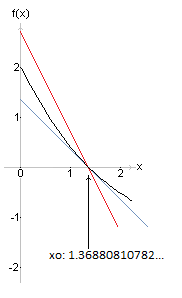
… and for greater value on n the result in 12 digit remains the same. The convergence is very fast and in only four iterations we have obtained the result of Fibonacci. Regarding the $\displaystyle a_{n}$ we observe that for n=0 the sequence increases and for greater n the sequence is decreasing. That is not a surprise if we observe the figure…

fig. 4.1

The ‘black line’ is $\displaystyle f(x)$, the ‘blue line’ is $\displaystyle g_{1}(x)=x_{0}-x$ and the ‘red line’ is $\displaystyle g_{2}(x)= 2\ (x_{0}-x)$ . If we observe with care we note that for $\displaystyle a_{0}$ in the region $\displaystyle x <x_{0}$ we are in the condition of theorem 4.2 and the convergence is oscillating and for $\displaystyle a_{0}$ in the region $\displaystyle x>x_{0}$ we are in the condition of theorem 4.1 and the convergence is monotonic and that is true for all possible values of $\displaystyle a_{0}$. In other words the Newton's method, applied to the Fibonacci’s equation, always converges no matter which is $\displaystyle a_{0}$. Unfortunately not always that is true, as we will see in next example.

We want to apply the Newton's method to the equation…

$\displaystyle \varphi(x)= \sin x=0$ (4.12)

Of course we know that $\displaystyle x=0$ is a solution of (4.12), but what we are interested for is to verify the convergence of the method. First we compute f(x) with (4.9)…

$\displaystyle f(x)= -\tan x$ (4.13)

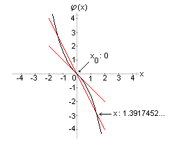
...and then we observe the diagram of f(x)…

fig. 4.2

Also in this case the is the ‘black line’ is f(x), the ‘blue line’ is $\displaystyle g_{1}(x)= x_{0}-x$ and the ‘red line’ is $\displaystyle g_{2}(x)=2 (x_{0}-x)$. For $\displaystyle –a<a_{0}<a$ where $\displaystyle a=1.3917452…$ we are in the conditions of theorem 4.2 and the Newton’s sequence will converge to the attractive fixed point $\displaystyle x_{0}=0$ with oscillations. For $\displaystyle a_{0}<-a$ or $\displaystyle a_{0}>a$ the convergence criterions of the theorem 4.1 or 4.2 aren’t satisfied and the Newton’s sequence will diverge. Before to proceed to the next section it is useful to apply the procedure now described to a very popular biological mathematical model: the inhibited growth model. According to this model, the population of a bacteria colonial grows according to the solution of the difference equation…

$\displaystyle \Delta_{n}=a_{n+1}-a_{n}= \beta\ a_{n}\ (1-\frac{a_{n}}{M})\ ;\ a_{0}=a$ (4.14)

… where $\displaystyle \beta$ is the ‘natural’ bacteria grow rate, i.e. the grow rate without any constraint, and M is the maximum number of bacteria that the ‘environmental resources’ can permit. If we ‘normalize’ the independent variable to M the f(x) in this case is…

$\displaystyle f(x)=\beta\ M\ x\ (1-x)$ (4.15)

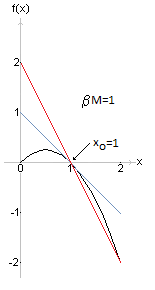
Using the described procedure we can identify two ‘critical values’ of the constant $\displaystyle \beta M$. For $\displaystyle \beta M=1$ f(x) is illustrated in fig. 4.3…

fig. 4.3

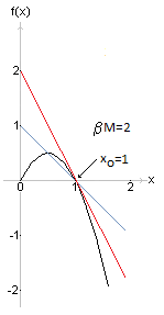
As in the previous cases the ‘black line’ isf(x), the ‘blue line’ is $\displaystyle g_{1}(x)= x_{0}-x$ and the ‘red line’ is $\displaystyle g_{2}(x)=2 (x_{0}-x)$. For $\displaystyle 0<a_{0}<1$ we are in the conditions of theorem 4.1 and the sequence will converge to the attractive fixed point $\displaystyle x_{0}=0$ ‘monotonically increasing’. The same is for $\displaystyle 0< \beta M< 1$. For $\displaystyle \beta M=2$ f(x) is illustrated in fig. 4.4…

fig. 4.4

Again the ‘black line’ is f(x), the ‘blue line’ is $\displaystyle g_{1}(x)= x_{0}-x$ and the ‘red line’ is $\displaystyle g_{2}(x)=2(x_{0}-x)$. For $\displaystyle 0<a_{0}<1$ we are in the conditions of theorem 4.2 and the sequence will converge to the attractive fixed point $\displaystyle x_{0}=0$ ‘oscillating’. The same is for $\displaystyle 1< \beta M< 2$. For $\displaystyle \beta M> 2$ the solution of the difference equation (4.15) will diverge no matter which is $\displaystyle a_{0}$ …

 

[chisigma]

5. Linear first order difference equations

Now we will have a look at the difference equation…

$\displaystyle a_{n+1}=\alpha_{n}\ a_{n}+\beta_{n}\ ;\ a_{0}=a$ (5.1)

Here $\displaystyle a_{n+1}$ is a linear function of the $\displaystyle a_{n}$ so that the (5.1) is a linear difference equation. Of course the $\displaystyle \alpha_{n}$ and the $\displaystyle \beta_{n}$ are in general discrete functions of n. Proceeding in ‘direct way’ from the initial value $\displaystyle a_{0}=a$ we find…

$\displaystyle a_{1}=\alpha_{0}\ a + \beta_{0}$

$\displaystyle a_{2}=\alpha_{0}\ \alpha_{1}\ a + \alpha_{1}\ \beta_{0}+ \beta_{1}$

$\displaystyle a_{3}=\alpha_{0}\ \alpha_{1}\ \alpha_{2}\ a + \alpha_{1}\ \alpha_{2}\ \beta_{0} + \alpha_{2}\ \beta_{1} + \beta_{2}$
...
Now if we set $\displaystyle p_{n}=\alpha_{0}\ \alpha_{1}\ …\ \alpha_{n-1}$, the solution can be written as…

$\displaystyle a_{n}= p_{n}\ (a+\frac{\beta_{0}}{p_{1}} + \frac{\beta_{1}}{p_{2}}+ … + \frac{\beta_{n-1}}{p_{n}} )$ (5.2)

As we said before, such result is not always full satisfactory and, when possible, an explicit solution as function of n is preferable. That is feasible in a large quantity of cases and we can start describing the simplest one: the case $\displaystyle \alpha_{n}= \alpha= \text{const}\ ,\ \beta_{n}=0$ , so that the difference equation is in the form…

$\displaystyle a_{n+1}= \alpha\ a_{n}\ ;\ a_{0}=a$ (5.3)

As for linear differential equations, a linear difference equation written as the (5.3) is called homogeneous and in this case the coefficients are constant. The solution is immediately derived from (5.2)…

$\displaystyle a_{n}= a\ \alpha^{n}$ (5.4)

This case is very simple but is of fundamental importance for the solution of more complex difference equations. The next step is to set $\displaystyle \alpha_{n}=\alpha=\text{const}$ and $\displaystyle \beta_{n}=\beta=\text{const}$, so that the difference equation is…

$\displaystyle a_{n+1}=\alpha\ a_{n}+\beta\ ;\ a_{0}=a$ (5.5)

As for linear differential equations, a linear difference equation written as the (5.5) is called nonhomogeneous. The solution is derived from (5.2) in a way a little more complex respect to the previous case…

$\displaystyle a_{n}=a\ \alpha^{n}+\beta\ \frac{1-\alpha^{n}}{1-\alpha}$ (5.6)

The (5.6) allows us to arrive to another important analogy between difference equations and differential equations: the solution of a nonhomogeneous difference equation is the sum of the solution of the homogeneous equation and ‘another term’ which doesn’t depend from the ‘initial value’ a… and the same is true also for higher order linear difference equations.

Now we perform a further step setting $\displaystyle \alpha_{n}=x$, $\displaystyle \beta_{n}=c_{n+1}$ and $\displaystyle a=c_{n}$, so that the difference equation is…

$\displaystyle a_{n+1}= x\ a_{n} + c_{n+1}\ ;\ a_{0}=1$ (5.7)

The solution, as derived from (5.2), is…

$\displaystyle a_{n}= \sum_{k=0}^{n}c_{n-k}\ x^{k}$ (5.8)

… and immediately we observe that it is a polynomial. The Horner method to compute a polynomial using only addictions and multiplications is based on the difference equation (5.7).

Proceeding with examples more and more complex we now examine the difference equation…

$\displaystyle a_{n+1}= \frac{n+1}{x}\ a_{n}+1\ ;\ a_{0}=1$ (5.9)

In (5.2) we have…

$\displaystyle p_{n}= \frac{n!}{x^{n}}$

... and for all n is $\displaystyle \beta_{n}=1$, so that the solution is…

$\displaystyle a_{n}= \sum_{k=0}^{n} \frac{x^{k}}{k!}$ (5.10)

… and for n ‘large enough’ is…

$\displaystyle a_{n} \sim e^{x}$

As in the previous case the difference equation (5.9) permits the practical computation of $\displaystyle e^{x}$ using only addictions and multiplications. With proper modifications in (5.9) a similar procedure is allowable for sin x, cos x, sinh x, cosh x, etc…, and in most cases it is a more convenient way to compute these functions respect to the ‘standard’ series expansion. Also for functions that can written as ‘infinite product’ this type of approach can be very useful, as in the following example: let consider the linear homogeneous difference equation…

$\displaystyle a_{n+1}= \{1-\frac{x^{2}}{(n+1)^{2}}\}\ a_{n}\ ;\ a_{0}=1$ (5.11)

Here the $\displaystyle \beta_{n}$ are all 0, so that from (5.2) we derive…

$\displaystyle a_{n}= p_{n} = \prod_{k=1}^{n} (1-\frac{x^{2}}{k^{2}})$ (5.12)

… and is…

$\displaystyle \lim_{n \rightarrow \infty} a_{n}= \prod_{k=1}^{\infty}(1-\frac{x^{2}}{k^{2}})= \frac{\sin \pi x }{\pi x}$ (5.13)

In general the effective computation of a numerical ‘finite or infinite’ sum can be reduced to the solution of a first order difference equation in the form…

$\displaystyle \Delta_{n}= a_{n+1}-a_{n}= \beta_{n}\ ;\ a_{0}=a$ (5.14)

… that is the general expression (5.1) where all the $\displaystyle \alpha_{n}$ are 0. An useful preliminary is the definition of the following function…

$\displaystyle \phi(x)=x\ \sum_{k=1}^{\infty} \frac{1}{k\ (k+x)} + c$ (5.15)

… where c is a constant that for the moment is left undefined. From (5.15) we derive immediately the ‘fundamental identity’…

$\displaystyle \phi(1+x)-\phi(x)= \sum_{k=1}^{\infty}\{\frac{1+x}{k\ (k+1+x)}-\frac{x}{k\ (k+x)}\}=$

$\displaystyle = \sum_{k=1}^{\infty}\{\frac{1}{k+x}-\frac{1}{k+1+x}\}= \frac{1}{1+x}$

… so that is…

$\displaystyle \phi(1+x)=\phi(x)+\frac{1}{1+x}$ (5.16)

The ‘fundamental identity’ (5.16) remember a property of the so called factorial function, defined as…

$\displaystyle x!=\int_{0}^{\infty} t^{x}\ e^{-t}\ d t$ (5.17)

Integrating by parts (5.17) we arrive to write…

$\displaystyle (1+x)!=x!\ (1+x)$ (5.18)

Now deriving (5.18) we obtain…

$\displaystyle \frac{d}{dx} (1+x)!=x!+\frac{d}{dx} x!\ (1+x)$

… so that is…

$\displaystyle \frac{\{(1+x)!\}^{‘}}{(1+x)!}= \frac{\{x!\}^{‘}}{x!}+ \frac{1}{1+x}$ (5.19)

It is easy to verify that the expressions (5.16) and (5.19) are ‘formally identical’ and that permits us to conclude that is…

$\displaystyle \phi(x)= \frac{d}{dx} \ln x!$ (5.20)

The (5.20) permits us to find the value of the constant c in (5.15). Starting from the ‘infinite product expansion’ of the factorial function with little efforts we can obtain the following McLaurin expansion, valid for |x|<1…

$\displaystyle \ln x!= -\gamma x+\sum_{k=2}^{\infty}(-1)^{k}\ \zeta(k)\ \frac{x^{k}}{k}$ (5.21)

… where $\displaystyle \zeta(*)$ is the so called ‘Riemann Zeta function’ …

$\displaystyle \zeta(x)= \sum_{k=1}^{\infty}\frac{1}{k^{x}}\ ,\ |x|>1$ (5.22)

… and $\displaystyle \gamma$ is the so called ‘Euler’s constant’…

$\displaystyle \gamma= \lim_{n \rightarrow \infty} (\sum_{k=1}^{n}\frac{1}{k}-\ln n)= .577215664901…$ (5.23)

Deriving the (5.21) we obtain…

$\displaystyle \frac{d}{dx} \ln x!= - \gamma + \sum_{k=2}^{\infty}(-1)^{k}\ \zeta(k)\ x^{k-1}$ (5.24)

… and comparing (5.15),(5.20) and (5.24) we conclude that the constant term in (5.15) and (5.24) must be the same and that in (5.15) is $\displaystyle c=-\gamma$.

Now if we set in (5.16) x=n, we discover that the sequence $\displaystyle \phi(n)$ satisfies the difference equation…

$\displaystyle \Delta_{n}= a_{n+1}-a_{n}= \frac{1}{n+1}\ ;\ a_{0}=- \gamma$ (5.25)

… the solution of which is…

$\displaystyle a_{n}= \phi(n)= \sum_{k=0}^{n-1}\frac{1}{k+1} - \gamma$ (5.26)

If we remember the definition of the Euler’s constant, it is easy to see that for n ‘large enough’ is…

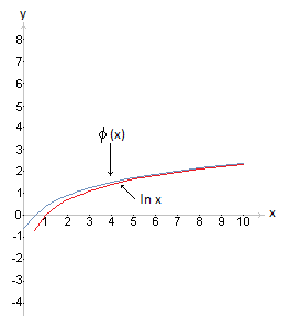
$\displaystyle \phi(n)\sim \ln n$ (5.27)

… and a ‘visible proof’ of that is illustrated in figure…

fig. 5.1

Although the term is used for more functions, we call the $\displaystyle \phi(*)$ we have defined in the last lines digamma function and now we illustrate in two examples how tom use its properties for the computation of finite or infinite sums. The first is the computation of…

$\displaystyle \sigma(n,t)= \sum_{k=1}^{n}\frac{1}{k+t}$ (5.28)

… for any value of n and t. If in (5.16) we set x=k+t-1 we obtain…

$\displaystyle \frac{1}{k+t}=\phi(k+t)-\phi(k+t-1)$

… so that the (5.28) can be treated as a telescopic sum and obtain…

$\displaystyle \sigma(n,t)= \sum_{k=1}^{n}\{\phi(k+t)-\phi(k+t-1)\}= \phi(n+t)-\phi(t)$ (5.29)

The second is the computation of the ‘infinite sum’…

$\displaystyle \sigma(a,b)= \sum_{k=1}^{\infty}\frac{1}{(k+a)\ (k+b)}$ (5.30)

… for any value of a and b. Writing the n-th partial sum of (5.30) taking into account (5.29) we have…

$\displaystyle \sigma_{n}= \sum_{k=1}^{n}\frac{1}{(k+a)\ (k+b)}= \frac{1}{b-a}\ \sum_{k=1}^{n}(\frac{1}{k+a}-\frac{1}{k+b})=$

$\displaystyle =\frac{1}{b-a}\ \{\phi(n+a)-\phi(a)-\phi(n+b)+\phi(b)\}$ (5.31)

A consequence of (5.27) is…

$\displaystyle \lim_{n \rightarrow \infty} \{\phi(n+a)-\phi(n+b)\}=0$

... so that we arrive to write…

$\displaystyle \sum_{k=1}^{\infty}\frac{1}{(k+a)\ (k+b)}= \frac{\phi(b)-\phi(a)}{b-a}$ (5.32)

Of course the field of linear first order difference equation is much wider, but our scope is only to supply some solving method. To acquire more material the reader can consult the specialized literature.

 

[chisigma]

6. Nonlinear first order difference equations

If a nonlinear first order is written in the form (4.5), then ’almost always’ the procedure illustrated in section 4 shows the general character of the solution. If not, then the solving procedure, if it exist, must be found ‘case by case’. One possibility is the variable change as in the following example…

$\displaystyle a_{n+1}= \alpha_{n}\ \frac{a_{n}}{1+a_{n}}\ ;\ a_{0}=a\ne 0$ (6.1)

… where the $\displaystyle \alpha_{n}$ are function of n. Here the variable change $\displaystyle b_{n}=\frac{1}{a_{n}}$ conducts to the difference equation…

$\displaystyle b_{n+1}= \frac{1+b_{n}}{\alpha_{n}}\ ;\ b_{0}=\frac{1}{a_{0}}$ (6.2)

… which is linear, so that the procedures of the section 5 can be applied.

Among the infinite set of first order non linear difference equations we will focus our attention on the so called Quadratic Maps. A Quadratic Map is a first order difference equation of the form…

$\displaystyle a_{n+1}= \alpha_{2}\ a^{2}_{n} + \alpha_{1}\ a_{n} + \alpha_{0}\ , a_{0}=a$ (6.3)

… where the $\displaystyle \alpha_{k}\ ,\ k=0,1,2$ are constants. Only a limited number of quadratic maps have solution in closed form. The simplest case is when only the quadratic term is $\displaystyle \ne 0$...

$\displaystyle a_{n+1}= \alpha_{2}\ a^{2}_{n}\ ,\ a_{0}=a$ (6.4)

… and the solution is…

$\displaystyle a_{n}= \alpha^{2^{n}-1}_{2}\ a^{2^{n}}$ (6.5}

The possibility of closed form solution however is much reduced if we add to the quadratic term a constant term. A well known example of that type of quadratic map is…

$\displaystyle a_{n+1}=a^{2}_{n}+c\ ;\ a_{0}=a$ (6.6)

… which defines the so called Mandelbrot set, and we will use it as ‘test model’, in the sense that the result obtained for it are obtainable [in principle…] for all the quadratic maps. The (6.6) in general doesn’t have a closed form solution. If we write the (6.6) as difference equation…

$\displaystyle \Delta_{n}=a_{n+1}-a_{n}= a^{2}_{n}-a_{n}+c= f(a_{n})$ (6.7)

… with the procedure illustrated in section 4 we find the two ‘fixed points’ [one ‘attractive fixed point’ $x_{1}$ and one ‘repulsive fixed point’ $x_{2}$…] as solution of the equation $\displaystyle f(x)=0$ i.e. …

$\displaystyle x_{1,2}= \frac{1 \pm \sqrt{1-4\ c}}{2}$ (6.8)

Proceeding as in section 4 we are able to find the set of ‘initial conditions’ that produce a sequence converging at $x_{1}$ or diverging from it and the task is left to the reader. Now our goal is finding closed form solutions of the (6.6). The search is in two phases and first we look at periodic solutions. Setting in (6.6) $\displaystyle a_{0}=x_{i}\ ;\ i=1,2$ we clearly obtain the solution $\displaystyle a_{n}=x_{i}\ ;\ i=1,2$, i.e. a constant sequence because is $\displaystyle a_{n+1}=a_{n}\ ,\forall n$. For that reason the $\displaystyle x_{i}\ ;\ i=1,2$ in (6.8) are called fixed points of periodicity 1. If we want to find solution with periodicity 2, then we have to impose the condition $\displaystyle a_{n+2}=a_{n}$ and that conducts to the equation…

$\displaystyle x^{4} +2\ c\ x^{2} – x +c\ (1+c)= (x^{2} –x +c)\ (x^{2} + x + 1+c)=0$ (6.9)

… that has solutions…

$\displaystyle x_{1,2}= \frac{1 \pm \sqrt{1-4\ c}}{2}\ ;\ x_{3,4}= \frac{-1 \pm \sqrt{-3-4 c}}{2}$ (6.10)

The $\displaystyle x_{i}\ ;\ i=1,2,3,4$ are called fixed points of periodicity 2. As expected the fixed points $x_{1,2}$ of periodicity 1 are also fixed point of periodicity 2 and in general if $\displaystyle k|n$ fixed point of periodicity k are also fixed points of periodicity n. In general the 2 k fixed points of periodicity k of (6.6) are found imposing the condition $\displaystyle a_{n+k}=a_{n}$ but of course the computational complexity greatly increases with k.

The second phase is the search of closed form non periodic solution of a quadratic map. Closed form solutions of the (6.3) do exist if we impose conditions on the $\displaystyle \alpha_{k}\ ;\ k=0,1,2$. We will illustrate two cases…

a) $\displaystyle \alpha_{0}= \frac{(\alpha_{1}-4)\ (\alpha_{1}+2)}{4\ \alpha_{2}}$ (6.11)

The solution of (6.3) is…

$\displaystyle a_{n}= \frac{r^{2 n} + r^{- 2 n} - \frac{\alpha_{1}}{2}}{\alpha_{2}}$ (6.12)

… where…

$\displaystyle r= \frac{\alpha_{1} + 2\ a\ \alpha_{2} + \sqrt{(2\ a\ \alpha_{2}+ \alpha_{1} +4)\ (2\ a\ \alpha_{2}+ \alpha_{1} -4)}}{4}$ (6.13)

Setting in (6.6) $\displaystyle c=-2$ the conditions in a) are satisfied giving…

$\displaystyle r= \frac{a}{2} + \sqrt{(\frac{a}{2})^{2}-1}$

$\displaystyle a_{n}= 2\ \cosh \{2\ n\ \ln [\frac{a}{2} + \sqrt{(\frac{a}{2})^{2}-1}]\}$ (6.14) b) $\displaystyle \alpha_{0}= \frac{\alpha_{1}\ (\alpha_{1}-2)}{4\ \alpha_{2}}$ (6.15)

The solution is…

$\displaystyle a_{n}= \frac{(2\ r)^{2^{n}}- \frac{\alpha_{1}}{2}}{\alpha_{2}}$ (6.16)

… where…

$\displaystyle r= \frac{\alpha_{1}+ 2\ a\ \alpha_{2}}{4}$ (6.17)

Setting in (6.6) $c=0$ the conditions in b) are satisfied and the solution is given by the (6.5) with $\displaystyle \alpha_{2}=1$.

The space limitation doesn’t allow us to do more and the interested reader is recommended to access to specialized licterature…