amjad-sh
- 240
- 13
In a single slit diffraction experiment, when we want to calculate the intensity of light on a screen located very far away from the slit, usually Huygens' principle is adopted as a model to perform the calculations.
It is assumed that the width of the slit consists of an infinite number of Huygens' sources, where each Huygens' source is a source of electromagnetic radiation that spreads in all directions. The interference of all the electromagnetic radiation emanating from all the sources creates the diffraction pattern that we see on the screen.
But what is confusing me is that the principle is only applied at the wave front that is present at the slit.
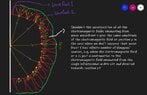
For example, suppose that the single-slit has an infinitesimal width. Therefore, the slit itself would be a Huygens' source. The Huygens' source will create a wave front and this initial wave front contains infinite number of Huygens' sources, and all of these infinite number of Huygens' sources will create their own wave front and so on.
I think in all textbooks, they don't take the electromagnetic field emanating from the other wave fronts ( the wave front that is not present at the slit) into account in summing up the electromagnetic radiation to get the intensity at a certain position. Shouldn't we take them into consideration to calculate the intensity? or is there a proof that the superposition of all the electromagnetic fields emanating from wave wave front 1 creates electromagnetic field at position p (on wave front 2 just after wave front 1) with an amplitude just equal to the amplitude of the electromagnetic field there but in the case when we don't suppose that wave front 1 has infinite number of Huygens'
sources, e.g., when the electromagnetic field at p is just a continuation to the electromagnetic field emanated from the single infinitesimal-width slit and directed towards position p?
See the attachment below for more clarification to my question.
It is assumed that the width of the slit consists of an infinite number of Huygens' sources, where each Huygens' source is a source of electromagnetic radiation that spreads in all directions. The interference of all the electromagnetic radiation emanating from all the sources creates the diffraction pattern that we see on the screen.
But what is confusing me is that the principle is only applied at the wave front that is present at the slit.
For example, suppose that the single-slit has an infinitesimal width. Therefore, the slit itself would be a Huygens' source. The Huygens' source will create a wave front and this initial wave front contains infinite number of Huygens' sources, and all of these infinite number of Huygens' sources will create their own wave front and so on.
I think in all textbooks, they don't take the electromagnetic field emanating from the other wave fronts ( the wave front that is not present at the slit) into account in summing up the electromagnetic radiation to get the intensity at a certain position. Shouldn't we take them into consideration to calculate the intensity? or is there a proof that the superposition of all the electromagnetic fields emanating from wave wave front 1 creates electromagnetic field at position p (on wave front 2 just after wave front 1) with an amplitude just equal to the amplitude of the electromagnetic field there but in the case when we don't suppose that wave front 1 has infinite number of Huygens'
sources, e.g., when the electromagnetic field at p is just a continuation to the electromagnetic field emanated from the single infinitesimal-width slit and directed towards position p?
See the attachment below for more clarification to my question.