I Impact of atmospheric turbulence on secret key rate in QKD

[Nur Ziadah]

TL;DR Summary

Clarification on the calculation of SKR over turbulence channel.

I have the calculation on secret key rate over the turbulence channel using Python code. The calculation is as below:

import numpy as np
import math
import re
import random
import cmath 
#import itertools
from math import pi,e,log
import time
#import xlwt
import matplotlib.pyplot as plt
from scipy.interpolate import splinex=np.linspace(0,1,1000)

def log_normal(x,sigma):
    y=1/(x*sigma*np.sqrt(2*np.pi))*np.exp(-(np.log(x/0.3)+(1/2*sigma*sigma))**2/(2*sigma*sigma))

    return ydef R(x,nd,Y0,ed):
    nsys = x*nd
    QBER=((1/2*Y0)+(ed*nsys))/(Y0+nsys)
    H2=-QBER*np.log2(QBER)-(1-QBER)*np.log2(1-QBER)
    out = (Y0+nsys)*(1-(2*H2))
    return outdef out(x,nd,Y0,ed,sigma):

    term1 = log_normal(x,sigma)
    term2 = R(x,nd,Y0,ed)

    return term1*term2

hyp = (0.25,1*(10**-5), 0.03,0.9) #nd,Y0,ed,sigmalg = log_normal(x[1:],hyp[3])

r = R(x[1:],hyp[0],hyp[1],hyp[2])
plt.plot(np.log10 ( out(x,hyp[0],hyp[1],hyp[2],0.9) ),label = "sigma = 0.9" )
plt.plot(np.log10 ( out(x,hyp[0],hyp[1],hyp[2],0.3) ) ,label = "sigma = 0.3")
plt.plot(np.log10 ( out(x,hyp[0],hyp[1],hyp[2],0.6) ) ,label = "sigma = 0.6")

plt.title("Rate")
plt.legend()
plt.show()

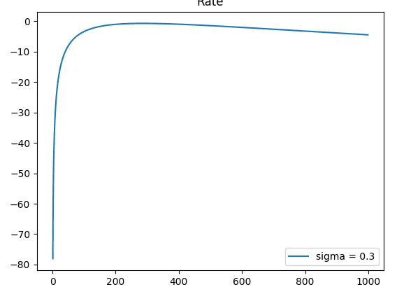
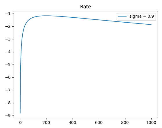
Theoretically, the SKR is low in high turbulence (sigma=0.9) and the SKR is high in low turbulence (sigma=0.3). However, after I ran this code, I get the wrong plot:

From the graphs, it can be seen at y-axis that the SKR under strong turbulence is higher compared to weak turbulence and vice versa. What is the problem in my calculation? Anyone, please help me. Thank you.

 

[mfb]

I have no idea about the underlying physics but the result fits to the code you wrote.

R is the same in both cases, let's focus on log_normal(x,sigma), especially the exponential function there:

exp(-(np.log(x/0.3)+(1/2*sigma*sigma))**2/(2*sigma*sigma))
Formatted:
$$\exp\left(\frac{-(\log(x/0.3)+1/2 \,\sigma^2)^2}{2\sigma^2}\right)$$
Your x range is from 1 to 1000, let's look at 300 for example: 300/0.3 = 1000, log(1000)=3. Plug it in and simplify a bit:
$$\exp\left(\frac{-(6+\sigma^2)^2}{8\sigma^2}\right)$$ As $\sigma<1$ we can neglect the right term and get approximately $$\exp\left(\frac{-36}{8\sigma^2}\right)$$
For small $\sigma$ the exponent is very large (here is a plot) and the expression is very small.

 

[Nur Ziadah]

I have no idea about the underlying physics but the result fits to the code you wrote.

R is the same in both cases, let's focus on log_normal(x,sigma), especially the exponential function there:

exp(-(np.log(x/0.3)+(1/2*sigma*sigma))**2/(2*sigma*sigma))
Formatted:
$$\exp\left(\frac{-(\log(x/0.3)+1/2 \,\sigma^2)^2}{2\sigma^2}\right)$$
Your x range is from 1 to 1000, let's look at 300 for example: 300/0.3 = 1000, log(1000)=3. Plug it in and simplify a bit:
$$\exp\left(\frac{-(6+\sigma^2)^2}{8\sigma^2}\right)$$ As $\sigma<1$ we can neglect the right term and get approximately $$\exp\left(\frac{-36}{8\sigma^2}\right)$$
For small $\sigma$ the exponent is very large (here is a plot) and the expression is very small.

Thank you for your explanation. ;)