Plotting a Bessel Function for Diffraction (Fraunhofer)

[PhDeezNutz]

Homework Statement

I want to plot formula 10.119 in Jackson

$\frac{dP}{d \Omega} \approx P_i \frac{\left(ka\right)^2}{4 \pi}\frac{\left(1 + \cos \theta \right)}{2}\left|\frac{J_1 \left( ka \sin \theta \right)}{ka \sin \theta} \right|^2$

(I have let $\alpha = 0$ for normal incidence)

Relevant Equations

See above

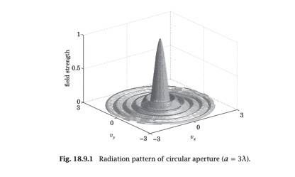
From my understanding of diffraction pattern is supposed to result in something like this

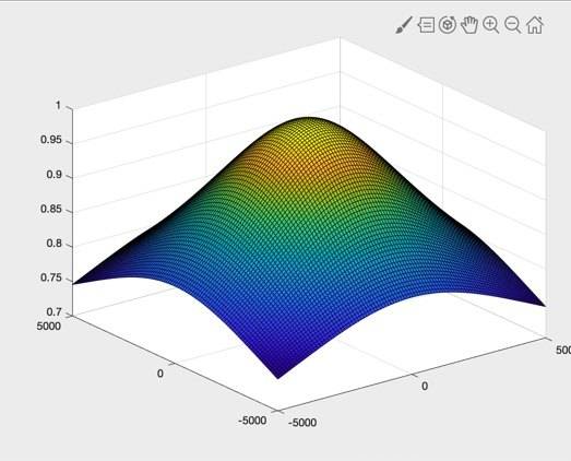
However when I plot it I get the central peak without the ripples (even when broadening the view). My result

My code is as follows %1) Define the grid. Define vectors so that they include 0, otherwise entire planes are excluded from the picture. We want only to exclude the% origin. Unfortunately there is no mechanism in place to ensure this with arbitrary choices. n = 100; rmax = 5000; x = linspace(-rmax,rmax,n); y = linspace(-rmax,rmax,n); z = linspace(-rmax,rmax,n); %2) Form a meshgrid and the first radial array [X,Y] = meshgrid(x,y); r = sqrt(X.^2 + Y.^2 + (z(90)*ones(size(Y))).^2); rnegative1 = r.^(-1); rnegative2 = r.^(-2); rnegative3 = r.^(-3); rnegative4 = r.^(-4); rnegative5 = r.^(-5);rnegative1(~isfinite(rnegative1)) = 0; rnegative2(~isfinite(rnegative2)) = 0; rnegative3(~isfinite(rnegative3)) = 0; rnegative4(~isfinite(rnegative4)) = 0; rnegative5(~isfinite(rnegative5)) = 0;r2 = sqrt(X.^2 + Y.^2); r2negative1 = r2.^(-1); r2negative2 = r2.^(-2); r2negative3 = r2.^(-3); r2negative4 = r2.^(-4); r2negative5 = r2.^(-5); r2negative1(~isfinite(r2negative1)) = 0; r2negative2(~isfinite(r2negative2)) = 0; r2negative3(~isfinite(r2negative3)) = 0; r2negative4(~isfinite(r2negative4)) = 0; r2negative5(~isfinite(r2negative5)) = 0;%3) Create constants k = 0.001*5*pi; epsilon = 8.85*(10^(-12)); c = 3*((10)^(8)); c1 = (4*pi)^(-1); c2= (4*pi*epsilon)^(-1);mu = (4*pi)*((10)^(-7)); omega = k*sqrt(mu*epsilon); E0 = 1; a = 1;%4) The kasintheta function r2 = sqrt(X.^2 + Y.^2); r3 = sqrt(X.^2 + Y.^2 + (z(90)*ones(size(Y))).^(2)); r3neg1 = r3.^(-1); kasintheta = k*a*r2.*((z(90)).^(-1)); kasinthetaneg1 = kasintheta.^(-1);Jfactor = (besselj(1,kasintheta).*kasinthetaneg1).^2; Jfactor(~isfinite(kasinthetaneg1)) = 0.25;Eratio = 2*((1+ z(90).*r3neg1).^2).*Jfactor; surf(X,Y,Eratio)

The part of the script that reads

Jfactor(~isfinite(kasinthetaneg1)) = 0.25; is to have a central peak instead of a central 0. It is a pathological case because $J_1$ has a zero at zero but $\frac{J_1 (x)}{x}$ has a peak at zero. Analogous to the sinc function.

Again I am getting a central peak but no ripple (not even tiny ones when I broaden my view).

Thanks for any help in advance. I'll probably have a bunch of follow up questions...fair warning :D

 

[PhDeezNutz]

I didn't believe the formulas given so I instead I graphed what I thought was reasonable for the poynting vector component going through the back screen.

$S_z = \frac{1}{z} \frac{J_1 \left(ka \sqrt{x^2 + y^2} \right) }{ka \sqrt{x^2 + y^2}}$

I figured $S_z$ had to depend on $z$ and had to decay as $z$ got bigger. Although my solution is qualitatively right I think it's wrong because I also think that the "period" should get bigger as $z$ gets bigger. (i.e. the wave gets more spread out).

 

[PhDeezNutz]

Turns out it is the electric field (z-component flux) that causes the pattern on the back screen.

I'm using some formulas from this paper for a circular aperture.

https://iopscience.iop.org/article/10.1070/PU2002v045n05ABEH001091

Namely the Hertz vector potential at the top of section 6. Then computing the curl twice to get the electric field. Then extracting the z-component.

This is my result.

It's not quite there. Getting the middle peak with ripples but the ripples are not cylindrically symmetric. In general the interpolation is "jagged".

Does anyone think if I Fourier Transform this graph I'll get a typical "airy disk pattern"?