Solving the Initial Value Problem for a Wave Using the Forward Euler Method

In summary, the conversation discussed the use of different methods, such as the forward Euler method, trapezoid method, Heun's method, Runge-Kutta method, and Gauss-Legendre method, to solve an initial value problem. The conversation also touched on the importance of including the initial conditions in the code and how to check the accuracy of the results. Additionally, the conversation discussed plotting the values of $(x^n)^2+(y^n)^2$ on a graph.
  • #1
evinda
Gold Member
MHB
3,836
0
Hello! (Wave)

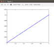
We consider the initial value problem

$$x'(t)=-y(t), t \in [0,1] \\ y'(t)=x(t), t \in [0,1] \\ x(0)=1, y(0)=0$$

I want to solve approximately the above problem using the forward Euler method in uniform partition of 100 and 200 points.

I have written the following code in matlab:

Code:
N=100;
h=1/N;
y=zeros(N);
A=[0 -1;1 0];
for (i=1:100)
    y=(eye(N,N)+A*h)*y
    i=i+1;
end
y

Is my code right? (Thinking)
 
Mathematics news on Phys.org
  • #2
Hey evinda! (Smile)

The dimensions of A do not match eye(N,N), nor y.
Shouldn't it be eye(2)?

And where is the initial condition $x(0)=1, y(0)=0$?
Shouldn't we have y=[1;0] instead of y=zeroes(N)? (Wondering)
 
  • #3
You can check your work by solving the equations analytically. The equations are
x′(t)=−y(t) and y′(t)=x(t). Differentiating the first equation again, x'(t)= -y'(t)= -x. That is a linear ordinary differential equation with constant coefficients. The general solution is x(t)= A cos(t)+ B sin(t). y(t)= -x'(t)= A sin(t)- B cos(t).

The initial condition is x(0)= A= 1, y(0)= -B= 0.

x(t)= cos(t), y(t)= sin(t).
Check your values against that.
 
  • #4
I like Serena said:
Hey evinda! (Smile)

The dimensions of A do not match eye(N,N), nor y.
Shouldn't it be eye(2)?

And where is the initial condition $x(0)=1, y(0)=0$?
Shouldn't we have y=[1;0] instead of y=zeroes(N)? (Wondering)

Ah I see... So the correct code would be the following, right? (Blush)

Code:
N=1/100;
h=1/N;
y=[1;0];
A=[0 -1;1 0];
for (i=1:N)
      y=(eye(2)+A*h)*y;
      i=i+1;
end
y
Using the trapezoid method, the code would get the following form, right?
Code:
N=100;
h=1/N;
y=[1;0];
A=[0 -1;1 0];
for (i=1:N)
     y=inv(eye(2)-h/2*A)*(eye(2)+h/2*A)*y;
     i=i+1;
end
y
 
  • #5
evinda said:
Ah I see... So the correct code would be the following, right? (Blush)

Code:
N=1/100;
h=1/N;
y=[1;0];
A=[0 -1;1 0];
for (i=1:N)
      y=(eye(2)+A*h)*y;
      i=i+1;
end
y

The [M]i=i+1[/M] is redundant, but yes, that will give the Nth approximation of the Forward Euler method. (Nod)

evinda said:
Using the trapezoid method, the code would get the following form, right?
Code:
N=100;
h=1/N;
y=[1;0];
A=[0 -1;1 0];
for (i=1:N)
     y=inv(eye(2)-h/2*A)*(eye(2)+h/2*A)*y;
     i=i+1;
end
y

How did you get that? (Wondering)

If I apply Heun's method, also known as the Explicit trapezoidal rule, I get:
$$y_{i+1} = y+\frac h2\big[Ay+A(y+hAy)\big] = y+hAy + \frac{h^2}{2}A^2y$$
 
  • #6
I like Serena said:
The [M]i=i+1[/M] is redundant, but yes, that will give the Nth approximation of the Forward Euler method. (Nod)

Ah yes, nice! (Smirk)

I like Serena said:
If I apply Heun's method, also known as the Explicit trapezoidal rule, I get:
$$y_{i+1} = y+\frac h2\big[Ay+A(y+hAy)\big] = y+hAy + \frac{h^2}{2}A^2y$$

Ok. Then the code should look as follows, shouldn't it? (Thinking)

Code:
N=100;
h=1/N;
y=[1;0];
A=[0 -1; 1 0];
for (i=1:N)
      y=(eye(2)+h*A+h^2/2*A^2)*y;
end
y
 
  • #7
Yep.
And it's already pretty close to [M][cos(1);sin(1)][/M]. (Happy)
 
  • #8
I like Serena said:
Yep.
And it's already pretty close to [M][cos(1);sin(1)][/M]. (Happy)

You mean the solution y? How do we deduce this?

Using the Runge-Kutta method of fourth order, we have the following code, right?

Code:
N=100;
h=1/N;
y=[1;0];
A=[0 -1;1 0];
for (i=1:N)
      k1=A*y
      k2=A*(y+1/2*k1*h);
      k3=A*(y+1/2*k2*h);
      k4=A*(y+k3*h);
      y=y+1/6*(k1+2*k2+2*k3+k4)*h;
end
y
 
  • #9
evinda said:
You mean the solution y? How do we deduce this?

It's the solution to the initial value problem, isn't it?
It we substitute $x(t)=\cos t$ and $y(t)=\sin t$, it satisfies the conditions. (Thinking)

evinda said:
Using the Runge-Kutta method of fourth order, we have the following code, right?

Code:
N=100;
h=1/N;
y=[1;0];
A=[0 -1;1 0];
for (i=1:N)
      k1=A*y
      k2=A*(y+1/2*k1*h);
      k3=A*(y+1/2*k2*h);
      k4=A*(y+k3*h);
      y=y+1/6*(k1+2*k2+2*k3+k4)*h;
end
y

Yep. (Nod)
 
  • #10
I like Serena said:
It's the solution to the initial value problem, isn't it?
It we substitute $x(t)=\cos t$ and $y(t)=\sin t$, it satisfies the conditions. (Thinking)

Yes, it is. (Nod)

I like Serena said:
Yep. (Nod)

Nice... (Happy)

I also want to solve the problem using the Gauss-Legendre method, $q=2$, in uniform partition of 100 and 200 points.

Which is the formula of this method? I have looked for it in the internet, but I didn't find something helpful. (Nerd)
 
  • #11
evinda said:
I also want to solve the problem using the Gauss-Legendre method, $q=2$, in uniform partition of 100 and 200 points.

Which is the formula of this method? I have looked for it in the internet, but I didn't find something helpful. (Nerd)

Until now, I only knew of the Gauss–Legendre quadrature for integration.
Anyway, http://www.wseas.us/e-library/conferences/2006bucharest/papers/518-127.pdf?origin=publication_detail seems to explain how to use it for IVP's as a variant of Runge-Kutta, including a dedicated 2-point formula. (Thinking)
 
  • #12
I like Serena said:
Until now, I only knew of the Gauss–Legendre quadrature for integration.
Anyway, http://www.wseas.us/e-library/conferences/2006bucharest/papers/518-127.pdf?origin=publication_detail seems to explain how to use it for IVP's as a variant of Runge-Kutta, including a dedicated 2-point formula. (Thinking)

So the code will have the following form, right? (Thinking)

Code:
N=100;
h=1/N;
y=[1;0];
A=[0 -1;1 0];
a1=0.5*(1-1/sqrt(3));
a2=0.5*(1+1/sqrt(3));
for (i=1:N)
      k1=(A+a1*h*A^2)*y;
      k2=A*(y+a2*h*k1);
      y=y+h/2*(k1+k2);
end
y
 
  • #13
evinda said:
So the code will have the following form, right? (Thinking)

Code:
N=100;
h=1/N;
y=[1;0];
A=[0 -1;1 0];
a1=0.5*(1-1/sqrt(3));
a2=0.5*(1+1/sqrt(3));
for (i=1:N)
      k1=(A+a1*h*A^2)*y;
      k2=A*(y+a2*h*k1);
      y=y+h/2*(k1+k2);
end
y

Yep. (Nod)
 
  • #14
I like Serena said:
Yep. (Nod)

Great. (Blush) I also want to represent in common graphs the corresponding values of $(x^n)^2+(y^n)^2$.
So do we add at each of the above for-loops the command [M] plot(y(1)^2+y(2)^2)[/M] after the calculation of y? (Thinking)
 
  • #15
evinda said:
Great. (Blush) I also want to represent in common graphs the corresponding values of $(x^n)^2+(y^n)^2$.
So do we add at each of the above for-loops the command [M] plot(y(1)^2+y(2)^2)[/M] after the calculation of y? (Thinking)

Well, according to description of plot, we have:
plot(Y) creates a 2-D line plot of the data in Y versus the index of each value.

That means that the first time we get a plot of the first point at x-coordinate 1.
The second time that plot is replaced by a plot of a single point that is again at x-coordinate 1.
And so on, ending in the plot of a single point that corresponds to the last iteration.
That's not what we want, is it? (Worried)

To add to the plot instead of replacing it, we can call [M]hold on[/M].
And perhaps we should specify an x-coordinate of, say, [M]i*h[/M]? (Wondering)
 
  • #16
I like Serena said:
To add to the plot instead of replacing it, we can call [M]hold on[/M].
And perhaps we should specify an x-coordinate of, say, [M]i*h[/M]? (Wondering)

I haven't really understood how we use the command plot. Could you maybe explain it further to me? (Worried)
 
  • #17
evinda said:
I haven't really understood how we use the command plot. Could you maybe explain it further to me? (Worried)

Suppose we do:
Code:
N=100;
h=1/N;
y=[1;0];
A=[0 -1;1 0];
plot(0, y(1)^2+y(2)^2);
hold on;
for (i=1:N)
      y=(eye(2)+A*h)*y;
      plot(i*h, y(1)^2+y(2)^2);
end
hold off;
y

We use the plot(X,Y) command, which is described as:
plot(X,Y) creates a 2-D line plot of the data in Y versus the corresponding values in X.

Then the first plot command will create the plot and put one value in there at x-coordinate 0.
Calling [M]hold on[/M] means that we want to hold the plot, such that subsequent plot commands get added to the same plot until we call [M]hold off[/M]. Without it, the previous plot command would be discarded.
And [M]plot(i*h, y(1)^2+y(2)^2)[/M] plots the desired value at the corresponding x-coordinate, which is [M]x=i*h[/M].

The result is:
View attachment 8104
(Thinking)
 

Attachments

  • ForwardEulerPlot.png
    ForwardEulerPlot.png
    4.4 KB · Views: 61
  • #18
Alternatively, we could first gather all the data, and afterwards create the plot.
For instance with:
Code:
N=100;
h=1/N;
y=[1;0];
A=[0 -1;1 0];
tt=[0];
yy=[y];
for (i=1:N)
      y=(eye(2)+A*h)*y;
      tt=[tt, i*h];
      yy=[yy, y];
end
plot(tt, yy(1,:).^2+yy(2,:).^2);

The advantage is that we can easily add other graphs in the same plot.
For instance with the actual x and y values.
Or with the graphs for the other approximations. (Thinking)
 
  • #19
I like Serena said:
Suppose we do:
Code:
N=100;
h=1/N;
y=[1;0];
A=[0 -1;1 0];
plot(0, y(1)^2+y(2)^2);
hold on;
for (i=1:N)
      y=(eye(2)+A*h)*y;
      plot(i*h, y(1)^2+y(2)^2);
end
hold off;
y

We use the plot(X,Y) command, which is described as:
plot(X,Y) creates a 2-D line plot of the data in Y versus the corresponding values in X.

Then the first plot command will create the plot and put one value in there at x-coordinate 0.
Calling [M]hold on[/M] means that we want to hold the plot, such that subsequent plot commands get added to the same plot until we call [M]hold off[/M]. Without it, the previous plot command would be discarded.
And [M]plot(i*h, y(1)^2+y(2)^2)[/M] plots the desired value at the corresponding x-coordinate, which is [M]x=i*h[/M].

The result is:

(Thinking)

Ah I see... Like that we get the plot of the approximation of $x^2+y^2$ at each time $t_i=0+ih$, right?

- - - Updated - - -

I like Serena said:
Alternatively, we could first gather all the data, and afterwards create the plot.
For instance with:
Code:
N=100;
h=1/N;
y=[1;0];
A=[0 -1;1 0];
tt=[0];
yy=[y];
for (i=1:N)
      y=(eye(2)+A*h)*y;
      tt=[tt, i*h];
      yy=[yy, y];
end
plot(tt, yy(1,:).^2+yy(2,:).^2);

The advantage is that we can easily add other graphs in the same plot.
For instance with the actual x and y values.
Or with the graphs for the other approximations. (Thinking)

Could you explain to me the commands

[M]tt=[0];
yy=[y];[/M]

and

[M]tt=[tt, i*h];
yy=[yy, y]; [/M]

?

With tt=[0]; for example, how do we know that the 2-dimensionsal zero vector is meant?
 
  • #20
evinda said:
Ah I see... Like that we get the plot of the approximation of $x^2+y^2$ at each time $t_i=0+ih$, right?

Indeed. (Nod)

evinda said:
Could you explain to me the commands

[M]tt=[0];
yy=[y];[/M]

and

[M]tt=[tt, i*h];
yy=[yy, y]; [/M]

?

With tt=[0]; for example, how do we know that the 2-dimensionsal zero vector is meant?

It's not. (Shake)

[M]tt=[0][/M] creates a row vector of t-values with the single scalar value 0 in it.
[M]yy=[y][/M] creates a matrix of y-vectors with with the single column vector y in it.
[M]tt=[tt, i*h][/M] creates a new row vector by adding [M]i*h[/M] to the right of [M]tt[/M].
[M]yy=[yy, y][/M] creates a new matrix by appending the column vector [M]y[/M] to the right of the matrix [M]yy[/M].

Afterwards [M]yy[/M] contains all the iterations of [M]y[/M], and [M]tt[/M] contains the corresponding t-values. (Thinking)
 
  • #21
I like Serena said:
Indeed. (Nod)
It's not. (Shake)

[M]tt=[0][/M] creates a row vector of t-values with the single scalar value 0 in it.
[M]yy=[y][/M] creates a matrix of y-vectors with with the single column vector y in it.
[M]tt=[tt, i*h][/M] creates a new row vector by adding [M]i*h[/M] to the right of [M]tt[/M].
[M]yy=[yy, y][/M] creates a new matrix by appending the column vector [M]y[/M] to the right of the matrix [M]yy[/M].

Afterwards [M]yy[/M] contains all the iterations of [M]y[/M], and [M]tt[/M] contains the corresponding t-values. (Thinking)

Nice... Thank you very much! (Happy)
 

1. What is an initial value problem (IVP)?

An initial value problem is a type of mathematical problem that involves finding a function or set of functions that satisfy a given set of conditions, called the initial values. These conditions typically involve the value of the function(s) at a specific point or points in time.

2. What is the difference between an initial value problem and a boundary value problem?

The main difference between an initial value problem and a boundary value problem is the type of conditions given. In an initial value problem, the conditions are given at a single point or a small interval of time, while in a boundary value problem, the conditions are given at different points or intervals along the boundary of the problem domain.

3. What is the importance of initial value problems in science?

Initial value problems are of great importance in science as they allow us to model and analyze various natural phenomena and physical systems. They are widely used in fields such as physics, engineering, and economics to predict how a system will evolve over time based on its initial conditions.

4. What are some common methods for solving initial value problems?

Some common methods for solving initial value problems include analytical methods, such as separation of variables and Laplace transforms, as well as numerical methods, such as Euler's method and Runge-Kutta methods. The choice of method depends on the complexity of the problem and the desired level of accuracy.

5. What are the limitations of initial value problems?

One limitation of initial value problems is that they only provide information about the behavior of a system for a finite time interval, based on the given initial conditions. They also assume that the system is well-behaved and does not experience sudden changes or discontinuities. In some cases, boundary value problems may be a better approach for modeling certain systems.

Similar threads

  • General Math
2
Replies
38
Views
10K
  • General Math
Replies
2
Views
727
Replies
7
Views
2K
  • General Math
Replies
11
Views
1K
Replies
1
Views
1K
  • Engineering and Comp Sci Homework Help
Replies
2
Views
2K
Replies
2
Views
258
  • General Math
Replies
1
Views
1K
  • General Math
Replies
1
Views
2K
Back
Top