swraman
- 165
- 0
Ive read other threads on here about this and am still slightly confused about it. I did a little experiment; and I am hoping someone can help shed some light on the results. The experiment:
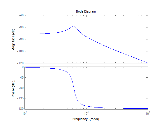
1. Create a system: modeled after a simple spring-mass-damper with mass=1 damping zeta=.1, natural frequency wn=2*pi*10,
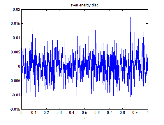
2. Create a PSD with uniform energy distribution (I chose to go to 500Hz, with a dF of 1). Paired this with a random phase, modified it so it had hermitian symmetry, and ifft'd that to get a time signal with an even energy distribution.
3. Apply this time signal to the Transfer function made in step 1. This will be the exact response to this system.
Now, I have a reference (generated in (2)) and a response of the system to (2). And, I can generate an FRF of the system from the reference and response I just measured:
H_FRF = fft(response) / fft(reference);
4. Now, I have a Fourier representation of the system taken from FFTs , as well as the laplace domain model it was generated from. Take the impulse response of both of these - in the TRF case by passing an impulse through it and in the FRF case by convolving with fft(impulse) and taking the ifft. Results below.
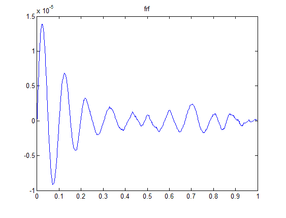
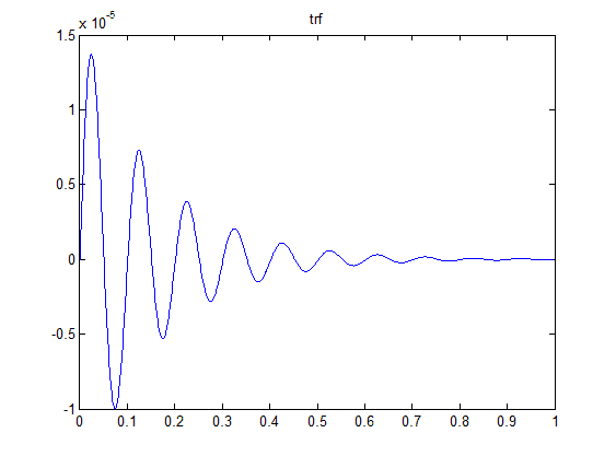
Clearly the Transfer function result is the correct result, but the FRF result is quite far off. Why is the FRF result so far off? I also added a few more averages (by generating more random time histories and responses) to my FRF, and the results don't change.
All the simulations were run at the same sample time with the same sample width; and as a result all FFTs were the same size; so leakage shouldn't be a problem. 500Hz is significantly higher than my resonance at 10Hz, so I don't suspect any aliasing effects to be in play.
Is it because (in a sense) dynamic systems are not represented well in the Fourier domain? That is, they can only be properly described in the laplace domain, in which a systems response to damped sine waves is also taken into account?
1. Create a system: modeled after a simple spring-mass-damper with mass=1 damping zeta=.1, natural frequency wn=2*pi*10,
2. Create a PSD with uniform energy distribution (I chose to go to 500Hz, with a dF of 1). Paired this with a random phase, modified it so it had hermitian symmetry, and ifft'd that to get a time signal with an even energy distribution.
3. Apply this time signal to the Transfer function made in step 1. This will be the exact response to this system.
Now, I have a reference (generated in (2)) and a response of the system to (2). And, I can generate an FRF of the system from the reference and response I just measured:
H_FRF = fft(response) / fft(reference);
4. Now, I have a Fourier representation of the system taken from FFTs , as well as the laplace domain model it was generated from. Take the impulse response of both of these - in the TRF case by passing an impulse through it and in the FRF case by convolving with fft(impulse) and taking the ifft. Results below.
Clearly the Transfer function result is the correct result, but the FRF result is quite far off. Why is the FRF result so far off? I also added a few more averages (by generating more random time histories and responses) to my FRF, and the results don't change.
All the simulations were run at the same sample time with the same sample width; and as a result all FFTs were the same size; so leakage shouldn't be a problem. 500Hz is significantly higher than my resonance at 10Hz, so I don't suspect any aliasing effects to be in play.
Is it because (in a sense) dynamic systems are not represented well in the Fourier domain? That is, they can only be properly described in the laplace domain, in which a systems response to damped sine waves is also taken into account?
Last edited: