Curve extrapolation: polynomial or Bézier?

[MisterH]

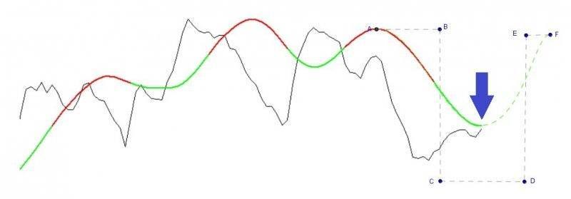
On a stationary, non-periodic signal (black) a smooth causal filter is calculated (green/red). It is sampled discretely (every distance unit of 1 on the X-axis). My goal is to find which "path" it is "travelling" on so I can extrapolate the current shape until it is completed (reaches a maximum/minimum: 1st derivative = 0), in real time: so at every point in time I assume the shape of the completed "path" and I want to measure the length between the previous turning point and the extrapolated turning point of this extrapolated curve:

I was playing around with a Geogebra script of a Bézier curve because dragging around the control points is visual and intuitive (for non-math guys like me) and it is easy to see where my current smooth movement would end if it were to continue "on the same path" it is currently on. I added some restrictions to my control polygon of my Bézier curve: 2 consecutive control points can only be on horizontal or vertical lines. In case of the image above, I used a Bézier curve of order 5, so it has 6 control points with the following restrictions:

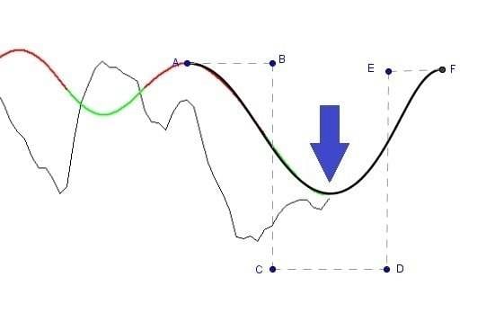
• A & B are on a horizontal line
• B & C are on a vertical line
• C & D are on a horizontal line
• D & E are on a vertical line
• E & F are on a horizontal line

So under these restrictions, at the blue arrow we assume the curve will continue via the dotted line to point F: so we start fitting the data from point A (the previous turning point) up to the blue arrow (a bit after the last turning point), and "extrapolate" further to F.

But then I realized that I don't need a parametric curve: I don't need an element of "speed" along the path (and all the headache that comes with that). I need something more simple. Should I just fit a polynomial

ax^5+bx^4+cx^3+dx^2+ex+f = 0

and then calculate where the slope of the tangent becomes 0 for points to the right of my blue arrow (to mimic that last control point F)? Or should I use a Bernstein polynomial to keep the same shape-properties as the Bézier, knowing that I only need y=f(x).

 

[FactChecker]

The first question that comes to my mind is to ask why you think that past history has any influence on the turning point (max or min) in the future? I certainly don't see any pattern. Some time series analysis might help to identify any relationship that would help you make a predictor. If time series analysis does not show a relationship, I think you may just be fooling yourself to make a predictor.

 

[MisterH]

My goal is not to use this signal as a predictor on itself: the data is only stationary, not periodic. I try to get an estimate for the instantaneous frequency of the smooth curve. This I can further use as an input for other filters and models that are calculated on the original signal so I can make those adaptive. Instead of using a look-back window of constant length, I change it dynamically. When the extrapolated turning-point lies further to the right of the last observation, I make the look-back window longer, if the extrapolated turning-point is at a short distance, my window length (of the other models) decreases.

 

[Svein]

1. Using polynomials is not recommended. Even if they fit your data points, they tend to oscillate wildly in between.
2. There are several families of orthogonal polynomials that are much better at approximation.
3. My personal favorite: Do a FFT of your data, throw away some of the highest frequencies and convert back.

 

[MisterH]

Using polynomials is not recommended. Even if they fit your data points, they tend to oscillate wildly in between.

Yes, probably related to Runge's[/PLAIN] Phenomenon?

My personal favorite: Do a FFT of your data, throw away some of the highest frequencies and convert back.

I am afraid that for online analysis, the FFT suffers from edge effect.

Something else I had in mind was this: the linearly swept sine / chirp: ( a sinusoidal wave that increases in frequency linearly over time):
Let me post some R-code of a linear chirp:

a<-1/100
b<-1/200
c<-1 #amplitude 1
d<-4
x<-1:80
output<-c*sin((pi/(b-a))*(((((x/d)*(b-a))+a)^2)-(a^2)))
plot(output,type="l",pch=20,lwd=3,col='orange',main="Chirp / Linearly Swept Sine & Bézier of order 5")

If I draw my Bézier curve of order 5 with the known restrictions on top of the linear chirp (from the first to the second to the last turning point), I see that they are equal: it is done manually, so there is some error on the estimation of the control points:

Maybe I could use the model of the linear chirp for the regression & extrapolation?
The code for the blue curve (Bézier curve of order 5) is this:

cpx<-c(8,40,40,65,65,78)
cpy<-c(output[8],output[8],-1.85,-1.85,output[78],output[78])

t<-seq(0,1,len=101)
P0<-matrix(data=c(cpx[1],cpy[1]),nrow=1,ncol=2,byrow=FALSE,dimnames=NULL)
P1<-matrix(data=c(cpx[2],cpy[2]),nrow=1,ncol=2,byrow=FALSE,dimnames=NULL)
P2<-matrix(data=c(cpx[3],cpy[3]),nrow=1,ncol=2,byrow=FALSE,dimnames=NULL)
P3<-matrix(data=c(cpx[4],cpy[4]),nrow=1,ncol=2,byrow=FALSE,dimnames=NULL)
P4<-matrix(data=c(cpx[5],cpy[5]),nrow=1,ncol=2,byrow=FALSE,dimnames=NULL)
P5<-matrix(data=c(cpx[6],cpy[6]),nrow=1,ncol=2,byrow=FALSE,dimnames=NULL)
par(mfrow=c(1,1),mar=c(2,2,2,0))
B<-(1-t)^5%*%P0+5*((1-t)^4)*t%*%P1+10*t^2*(1-t)^3%*%P2+10*(1-t)^2*t^3%*%P3+5*(1-t)*t^4%*%P4+t^5%*%P5
# plot(0,col="red",pch=20,type="n",xlim=c((min(cpx)-10),(max(cpx)+10)),ylim=c((min(cpy)-10),(max(cpy)+10)),main="Bézier Curve of 5th order")
plot(output,type="l",pch=20,lwd=3,col='orange',main="Chirp / Linearly Swept Sine & Bézier of order 5",ylim=c(-2,2));abline(h=0,lty=3)
lines(B,col='deepskyblue',lwd=3,lty=2)
points(P0,pch=20,col='deepskyblue');points(P1,pch=20,col='deepskyblue');points(P2,pch=20,col='deepskyblue');points(P3,pch=20,col='deepskyblue');points(P4,pch=20,col='deepskyblue');points(P5,pch=20,col='deepskyblue');text(cpx[1],cpy[1],"P0",cex=.8,pos=1,col='deepskyblue');text(cpx[2],cpy[2],"P1",cex=.8,pos=1,col='deepskyblue');text(cpx[3],cpy[3],"P2",cex=.8,pos=2,col='deepskyblue');text(cpx[4],cpy[4],"P3",cex=.8,pos=4,col='deepskyblue');text(cpx[5],cpy[5],"P4",cex=.8,pos=1,col='deepskyblue');text(cpx[6],cpy[6],"P5",cex=.8,pos=1,col='deepskyblue');segments(cpx[1],cpy[1],cpx[2],cpy[2],lty=3,col='deepskyblue');segments(cpx[2],cpy[2],cpx[3],cpy[3],lty=3,col='deepskyblue');segments(cpx[3],cpy[3],cpx[4],cpy[4],lty=3,col='deepskyblue');segments(cpx[4],cpy[4],cpx[5],cpy[5],lty=3,col='deepskyblue');segments(cpx[5],cpy[5],cpx[6],cpy[6],lty=3,col='deepskyblue')

 

[Svein]

I am afraid that for online analysis, the FFT suffers from edge effect.

Forgot to say, do a linear regression first and subtract that line. Then add it back at the end.

 

[FactChecker]

so I can extrapolate the current shape ... the extrapolated turning point of this extrapolated curve:

Are you sure you are not using this as a predictor?

 

[MisterH]

Are you sure you are not using this as a predictor?

I confess! I guess that I want to use it as an indirect predictor: a predictor for the length of the look-back window of another filter. Whether that is prediction or not is debatable/semantics. In my opinion trying to find the instantaneous frequency of a smooth curve by some extrapolation method is not really about prediction (which is about the future), but more about estimating the state/regime of the present.

 

[FactChecker]

more about estimating the state/regime of the present.

I understand now. I agree.