How are the equations of continuity derived in 1D?

[aliens123]

In Landau-Lifshitz Volume 6 Fluid-Mechanics the following problem is given

Where the equation of continuity is given earlier:

As is Euler's equation:

And the equation of continuity for entropy:

I don't understand how this conclusion was reached. I can understand the derivation for the equation of continuity , but I have no idea how you could derive it from Euler's equation:
$$ \frac{\partial \rho}{\partial t} + \nablda \cdot ( \rho} \vec{v} )=0 $$
In 1d:
$$ \frac{\partial \rho}{\partial t} + \frac{\partial }{\partial a} ( \rho} v )=0 $$
I tried integrating this with
$$\int_{t_0}^{t} dt$$: $$\rho - \rho_0 + \frac{\partial }{\partial a} \int_{t_0}^{t} \rho \frac{\partial x}{\partial t}dt = 0$$
But I can't see any way to simplify this...

I also do not see how the next two equations were derived. Any help would be appreciated.

 

[vanhees71]

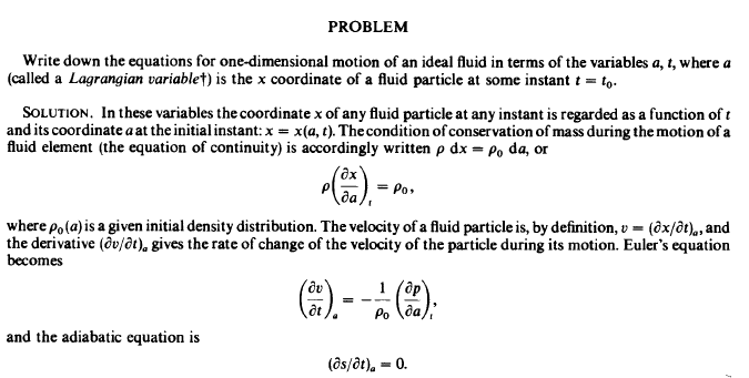
This is simply the transformation between Lagrange and Euler descriptions of the fluid.

In the Lagrange description you use some standard configuration of a continuum mechanical system. For fluids you can choose the configuration at the initial time $t$. Then one defines $\vec{x}(t,\vec{y})$ as the position of the fluid element at time $t$, which has been located at $\vec{y}$ at time $t=0$. We assume that the map $\vec{y} \mapsto \vec{x}(t,\vec{y})$ is smooth and invertible (a diffeomorphism).

Then the velocity of the fluid element is simply given by
$$\vec{v}_L(t,\vec{y})=\partial_t \vec{x}(t,\vec{y}).$$
That's the Lagrangian description of the fluid motion (and that's why I put an $L$ at the velocity).

The more familiar Eulerian description is found when thinking in terms of an observer looking at the fluid at position $\vec{x}$ and just describes the properties of the fluid element at time $t$ which is just at this position. Then you get the usual velocity field of fluid dynamics
$$\vec{v}(t,\vec{x})=\vec{v}_L[t,\vec{y}(t,\vec{x})],$$
where now we simply write $\vec{y}(t,\vec{x})$ for the inverse function of $\vec{x}(t,\vec{y})$, i.e., $\vec{y}(t,\vec{x})$ gives the initial $\vec{y}$ of the fluid element which is at $\vec{x}$ at time $t$.

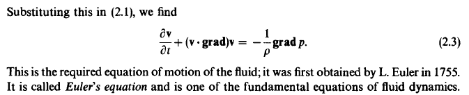
From this you get the acceleration of a given fluid element as follows: In Lagrangian description it's simply
$$\vec{a}_L(t,\vec{y})=\partial_t \vec{v}_L(t,\vec{y}),$$
but now we want to express this in the Eulerian description. To that end we note that
$$\vec{v}_L(t,\vec{y})=\vec{v}[t,\vec{x}(t,\vec{y})].$$
And then we get
$$\vec{a}_L(t,\vec{y})=\vec{a}(t,\vec{x})=\partial_t \vec{v}[t,\vec{x}(t,\vec{y})]=\partial t \vec{v}(t,\vec{x}) + [\partial_t \vec{x}(t,\vec{y}) \cdot \vec{\nabla} \vec{v}(t,\vec{x}) = \partial_t \vec{v}(t,\vec{x}) + (\vec{v} \cdot\vec{\nabla}) \vec{v}(t,\vec{x}).$$
This you can generalized to the "substantial time derivative" of any quantity, and define
$$\mathrm{D}_t f(t,\vec{x})=\partial_t f(t,\vec{x}) + (\vec{v} \cdot \vec{\nabla}) f(t,\vec{x}).$$
Now again consider a fixed fluid element at the initial position $\vec{y}$. Then the mass density in Lagrangian description is given by $\rho_L(t,\vec{y})$.

Now for these given fluid particles the mass is conserved, i.e.,
$$\mathrm{d} m = \mathrm{d}^3 x \rho_L=\text{const}. \; \Rightarrow \; \partial_t \mathrm{d} m=0.$$
The partial time derivative has to be taken with $\vec{y}$ fixed.

In terms of the Eulerian density we have
$$\mathrm{d} m=\mathrm{d}^3 x \rho=\mathrm{d}^3 \vec{y} \mathrm{det} \frac{\partial \vec{x}}{\partial \vec{y}} \rho=\mathrm{d}^3 \vec{y} J(t,\vec{y}) \rho_L(t,\vec{y}).$$
Here $J$ is the Jacobian of the diffeomorphism $\vec{y} \mapsto \vec{x}(t,\vec{y})$. The time derivative is given by
$$\partial_t J=(\vec{\nabla} \cdot \vec{v}) J.$$
From this you get
$$\partial_t \mathrm{d}m =\mathrm{d}^3 y J (\partial_t \rho_L(t,\vec{y}) + \rho_L \vec{\nabla} \cdot \vec{v}_L)=0.$$
Now we can rewrite this again in terms of the Eulerian description, using $\partial_t \rho_L=\mathrm{D}_t \rho$:
$$\mathrm{D}_t \rho + \rho \vec{\nabla} \cdot \vec{v}=0$$
or writing the material time derivative out
$$\partial_t \rho + (\vec{v} \cdot \vec{\nabla}) \rho + \rho \vec{\nabla} \cdot \vec{v} = \partial_t \rho +\vec{\nabla} \cdot (\rho \vec{v})=0.$$
This is the equation of continuity for the mass,
$$\partial_t \rho + \vec{\nabla} \cdot \vec{j},$$
where $\vec{j}=\rho \vec{v}$ is the mass-current density.

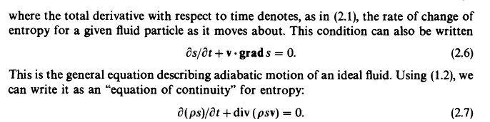
That the ideal fluid motion is adiabatic characterizes the ideal fluid which by definition does not dissipate energy into heat, i.e., the entropy per unit mass $s$ is constant for the corresponding fluid element, which means
$$\partial_t s_L(t,\vec{y})=\mathrm{D}_t s(t,\vec{x})=\partial_t s + (\vec{v} \cdot \vec{\nabla})s=0.$$
This only means that the entropy of each fluid element is conserved, indeed we have
$$\partial_t (\rho s) + \vec{\nabla} \cdot (\vec{j} s)=(\partial_t \rho + \vec{\nabla} \cdot \vec{j}) + \rho \partial_t s +(\vec{j} \cdot \vec{\nabla}) s=\rho (\partial_t s + \vec{v} \cdot \vec{\nabla} s)=0.$$