Modelling of two phase flow in packed bed using conservation equations

454 replies · 45K views · last reply
casualguitar said:
Hi Chet, have I got both the intended computational flow, and correlations to be used, correct here? The only change from he previous version was to include the new Nu correlation from BSL rather than from Dixon et al.

View attachment 297395

You mentioned your version gives Nu directly, and the previous version I did does not do that. I don't see where that comes into play here. Is this correct?
The BSL definitions of Nu and Re are different from these. So, if you use these equations, you will get the wrong answer for the convective heat transfer coefficient.
 
This is the approach using the BSL Re correlation (eq.2, or 14.5-4 in BSL). The Nu definition I used is the same though. This approach does allow you to get. Nu 'directly' as it cancels out as you mentioned. Have I used the correct Nu correlation here?
Handwritten notes on lined paper deriving packed bed correlations: Pr and Re definitions, Nu and jH relations, the Chilton-Colburn j-factor, and the expression for h in terms of h_fs, d_p, and k_f.
 
casualguitar said:
This is the approach using the BSL Re correlation (eq.2, or 14.5-4 in BSL). The Nu definition I used is the same though. This approach does allow you to get. Nu 'directly' as it cancels out as you mentioned. Have I used the correct Nu correlation here?
View attachment 297457
casualguitar said:
This is the approach using the BSL Re correlation (eq.2, or 14.5-4 in BSL). The Nu definition I used is the same though. This approach does allow you to get. Nu 'directly' as it cancels out as you mentioned. Have I used the correct Nu correlation here?
View attachment 297457
This version is correct, but different from the incorrect version you provided in post #389.
 
Chestermiller said:
This version is correct, but different from the incorrect version you provided in post #389.
Got it I see the difference. Great. I've implemented this in a separate script so I will add this U(T,P,m_dot) function into the main script now

You mentioned previously we should include the internal resistance of the solid particle in the lumped parameter model. Is this the bottom right term in eq.8 above?
 
casualguitar said:
Got it I see the difference. Great. I've implemented this in a separate script so I will add this U(T,P,m_dot) function into the main script now

You mentioned previously we should include the internal resistance of the solid particle in the lumped parameter model. Is this the bottom right term in eq.8 above?
Sure
 
Chestermiller said:
Sure
Ok this function is now integrated into the main model. I am getting some unusual output (not because of the new U function, I was getting it before that). My guess its a units thing so I'm going to do a full debug to see what is going on
 
Chestermiller said:
Sure
Hi Chet, I've done a 1st debug of the script and these are the output plots, which are definitely incorrect, however I'm sharing them anyway to show where the model is at. The S shaped curves are not as 'nice' as I expected. I think the source of the error is that I am mixing up the ICs/BCs for m and m_dot somewhere, however that's just a guess for now
Line plot titled 'm dot for all tanks' of mass flow (mol/s) against time from 0 to 2000 for tanks 1 to 3, with dashed and dash-dot lines; flows stay near zero, then rise to about 8 mol/s near time 1350 and spike to about 148 mol/s near time 1450.
Line plot titled 'Fluid temperature for all tanks' showing fluid temp against time from 0 to 2000 for three tanks; tank 1 rises steadily to about 140, tanks 2 and 3 stay near 80 until a sharp jump around time 1400.
Line plot titled Mass hold up for all tanks, with Time on the x-axis from 0 to about 2000 and Mass hold up (mol) on the y-axis from about 20 to 140. Three curves for tank 1, tank 2 and tank 3 start near 139 mol and decline, with the drop steepening sharply after roughly time 1350 to 1500.

Line graph titled 'h for all tanks' of h (J/mol) against Time from 0 to 2000 for tank 1 h, tank 2 h and tank 3 h; all curves start near -12,200 and end between -6,400 and -5,600, with a steep rise between about 1350 and 1550.
 
Attachments
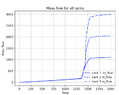
  • Line graph titled Mass flow for all tanks, plotting mass flow against time from 0 to 2000 for tanks 1, 2 and 3; all three curves rise slowly until about 1350, then jump sharply and level off near 1100, 2050 and 2990.
    Screenshot 2022-02-23 at 15.01.46.png
    16.6 KB · Views: 196
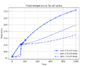
  • Line plot titled 'Fluid temperature for all tanks', fluid temp against time from 0 to 1000; tank 1 rises steadily to about 255, tanks 2 and 3 rise more slowly, with a sharp jump near time 140 for tank 2 and tank 3 leveling off near 125 to 130.
    Screenshot 2022-02-23 at 12.05.21.png
    20.6 KB · Views: 182
Hi Chet, apologies I'm actually still debugging. I think the bug is in the mass holdup and mass flow rate usage. I'm almost sure I'm not setting up the boundary and initial conditions correctly for these. The reason I think this is because 1) after thinking about it I'm actually not sure if I should use m or m_dot an an initial condition and 2) The plots above show n=1 as being shaped differently to the other positions

Its late here so I'll reframe this as both a question and a clear summary of how I am using m and mdot in the morning
 
casualguitar said:
Hi Chet, apologies I'm actually still debugging. I think the bug is in the mass holdup and mass flow rate usage. I'm almost sure I'm not setting up the boundary and initial conditions correctly for these. The reason I think this is because 1) after thinking about it I'm actually not sure if I should use m or m_dot an an initial condition and 2) The plots above show n=1 as being shaped differently to the other positions

Its late here so I'll reframe this as both a question and a clear summary of how I am using m and mdot in the morning
By the initial condition, you mean time zero, right? Why do you need this mdot?
 
Chestermiller said:
By the initial condition, you mean time zero, right? Why do you need this mdot?
The initial condition array is y0 = [h0,Ts0,m0, h1,Ts1,m1,...hn,Tsn,mn]
The solution array however is y = [h0,Ts0,mdot0, h1,Ts1,mdot1,...hn,Tsn,mdotn]

So I am supplying mass holdup as one of the initial conditions (mdot is only supplied as a boundary condition i.e. the inlet flow), and the solution array has mdot, not mass holdup

This is the code I am currently using:

Its a lengthy script, however it is just the my_system function where the algebraic solutions for each derivative at each position are set up that are important, and the few lines after this where the initial conditions are set up

I could put mass holdup in the solution array also, and then solve for mdot in the after processing stage. I don't know if this would affect the output though. I'll try this
 
casualguitar said:
The initial condition array is y0 = [h0,Ts0,m0, h1,Ts1,m1,...hn,Tsn,mn]
The solution array however is y = [h0,Ts0,mdot0, h1,Ts1,mdot1,...hn,Tsn,mdotn]

So I am supplying mass holdup as one of the initial conditions (mdot is only supplied as a boundary condition i.e. the inlet flow), and the solution array has mdot, not mass holdup

This is the code I am currently using:

Its a lengthy script, however it is just the my_system function where the algebraic solutions for each derivative at each position are set up that are important, and the few lines after this where the initial conditions are set up

I could put mass holdup in the solution array also, and then solve for mdot in the after processing stage. I don't know if this would affect the output though. I'll try this

What parameters are being integrated with respect to time (I.e.,your dependent variables)?
 
Chestermiller said:
What parameters are being integrated with respect to time (I.e.,your dependent variables)?
The parameters in the dydt list (in the script) are being integrated w.r.t. time and these are fluid enthalpy, solid temperature, and m_dot (mass flow rate out), which are equations 2, 3, and 4a in the image below (your original equations).

Now that you mention it, eq.2. and 3 have time derivatives, but 4a does not. We can solve directly for dm/dt and m_dot, so would I just need to integrate eq.2. and 3 here? I'm actually not sure why I assumed I would need to integrate 3 equations
Typeset equations (1) to (4b) for a packed bed of tanks: mass balance dm_j/dt = mdot_{j-1} - mdot_j, enthalpy balance m_j dh_j/dt = mdot_{j-1}(h_{j-1} - h_j) + UA_j(T_{S,j} - T_j), solid energy balance, and rearranged mass flow mdot_j = mdot_{j-1} - dm_j/dt.
 
Last edited:
casualguitar said:
The parameters in the dydt list (in the script) are being integrated w.r.t. time and these are fluid enthalpy, solid temperature, and m_dot (mass flow rate out), which are equations 2, 3, and 4a in the image below (your original equations).

Now that you mention it, eq.2. and 3 have time derivatives, but 4a does not. We can solve directly for dm/dt and m_dot, so would I just need to integrate eq.2. and 3 here? I'm actually not sure why I assumed I would need to integrate 3 equations
View attachment 297588
Yes, just two. The other equation is spatial only.
 
Chestermiller said:
Yes, just two. The other equation is spatial only.
Hi Chet, I have removed dm/dt from the dependent variables (required some small code adjustments to the after processing etc also). The simulation takes close to 10 minutes to run 1000s of simulation time, so this evening I am looking into optimising this code (replacing the nested for loop with a vectorised alternative, etc).

These are the plots produced by the simulation. They are not the 'perfect' S shaped curves I was thinking they might be. Do these curves look reasonable, or do they suggest there are further simulation errors? If the latter, would you have a suggestion as for how to systematically approach debugging?

Fluid enthalpy for 3 tanks:
Line plot titled 'h for all tanks' of h (J/mol) against Time from 0 to 1000 for tank 1 h, tank 2 h and tank 3 h; all three rise from about -12,200 J/mol, with a sharp jump near time 150 to about -6,500 J/mol, then rise more slowly, tank 1 highest at about -1,600 at time 1000.

Solid Temperature:
Line plot titled Solid Temperature for all tanks, Solid Temperature against Time from 0 to 1000 for three tanks. Tank 1 rises steadily to about 255; tanks 2 and 3 rise to about 198 and 162, with a sharp jump near time 140 to about 127.

Mass holdup for all tanks (note mole unit):
Line graph titled "Mass hold up for all tanks" plotting mass hold up (mol), from 0 to about 140, against time from 0 to 1000. Three curves start near 139 and drop sharply near time 140-160 to about 20-25, then decline slowly to about 8-16 by time 1000; tank 1 falls earlier and more gradually than tanks 2 and 3.

Fluid temperature (not reason for red plot here is I used two different approaches to calculate this, just checking that they are equivalent):
Line plot titled Fluid temperature for all tanks, Fluid temperature against Time from 0 to 1000, with three tanks shown in solid, dashed and dash-dot lines; all start near 80 and rise, with a sudden jump near time 140 and curves diverging afterward, tank 1 reaching about 255 at the end.

The main thing I am concerned about in these plots, is that the plot shape of the first tank is not the same as the other tanks, suggesting that I am possibly doing something wrong in how I am setting up the initial/boundary conditions
 
Last edited:
casualguitar said:
Hi Chet, I have removed dm/dt from the dependent variables (required some small code adjustments to the after processing etc also). The simulation takes close to 10 minutes to run 1000s of simulation time, so this evening I am looking into optimising this code (replacing the nested for loop with a vectorised alternative, etc).

These are the plots produced by the simulation. They are not the 'perfect' S shaped curves I was thinking they might be. Do these curves look reasonable, or do they suggest there are further simulation errors? If the latter, would you have a suggestion as for how to systematically approach debugging?

Fluid enthalpy for 3 tanks:
View attachment 297676
Solid Temperature:
View attachment 297677
Mass holdup for all tanks (note mole unit):
View attachment 297678
Fluid temperature (not reason for red plot here is I used two different approaches to calculate this, just checking that they are equivalent):
View attachment 297679
The main thing I am concerned about in these plots, is that the plot shape of the first tank is not the same as the other tanks, suggesting that I am possibly doing something wrong in how I am setting up the initial/boundary conditions
Check the 1st tank response against the 1 tank model with 1/n the volume.
 
  • Like
Likes   Reactions: casualguitar
Chestermiller said:
Check the 1st tank response against the 1 tank model with 1/n the volume.
Yes the plot for the 1 tank model is in the same ballpark as the full model (semi surprised that they line up this well). This is using an averaged value for the T dependent parameters like heat capacity. The constant temperature zone is more pronounced in the main model, however at all times the temperature discrepancy between the two models is fairly reasonable, which suggests that the main model does not set up the boundary/initial conditions incorrectly, suggesting that the model may be bug-free?
Line plot of Tf against t from 0 to 1000: a single blue curve rising from about 80 at t=0 to about 233 at t=1000, with a concave-down shape and grid lines.

There does remain the issue of the simulation taking a very long time to run. I am currently timing it but it is definitely 10+ minutes (EDIT: it took 15 mins to run to completion). It does look like there is something going on in the saturation zone where thermo takes a while to converge. If this can be fixed then simulation time will come down by a lot because the gas and liquid zones are relatively quick to simulate
 
Last edited:
Hi Chet, some short updates -

It is the thermo functions that are computationally expensive. I am looking into how these can be made less expensive to use for now (mostly to speed up model development)

We previously discussed tuning the model to experimental data. I have checked with the lab and the experimental data will be in excel format (straightforward to deal with from a programming point of view). Python has some nice curve fitting libraries that take x-y data, the model, and the tuning parameter(s), and return 'optimised' parameters using say least squares for example.

We discussed tuning parameters earlier on in the model (screenshot below is from post #99). This dispersivity parameter no longer seems to be accessible as it is not on the 'top layer' of the model anymore. Should this still be used as the tuning parameter, or are we now using another parameter that is at the top level of the model?
Two equations from a forum post: the continuity equation d(phi)/dt + d(phi)/dx = 0, and d(rho h)/dt + d(phi h)/dx = d/dx(phi l dh/dx) + Ua/epsilon (T_S - T), followed by text about the dispersivity parameter l.


And lastly, I have no model functionality left on my list that seems to be very important to implement (pressure gradient using relative permeability, internal particle temperature gradients). Do you see any functionality that should be implemented, before moving to the next section of this model (adding CO2 to the air mixture)?
Edit: Before moving forward, I will do a write up of everything we have discussed on the final version of the model tomorrow (late here now)
 
Hi Chet, short write up of the discussion we've had to date (on the most complex version of this model only so far) :https://docs.google.com/document/d/...ouid=111822275555236809516&rtpof=true&sd=true

The link is to a word doc of a summarised version of this discussion, plus output from the model and the actual Python script I made. I'll leave this link active indefinitely in case this is useful to any future passers by on this forum. I will also be updating it regularly until the packed bed modelling is finished so I'll probably change the location to an open google drive file

If it is ok with you I would like to discuss adding CO2 to the existing model. The idea here is that an ambient temperature air-CO2 mixture is passed through a cold packed bed, liquefying the air and freezing the CO2. The solid CO2 will move through the bed as a 'plug' which accumulates in mass as it passes through the bed, and will be extracted from the line at the end of the packed bed therefore 'cleaning' the air stream of CO2. If this is ok with you, I would like to attempt to lay out the mass and energy balances for this model (similar to what you did initially for the air model). I will definitely have questions on the mass balance for CO2, but I think it would be useful anyway to make an attempt so we have an initial discussion point!
 
Last edited:
Hi Chet, just posting the updated plots here. These plots include the heat transfer coefficient correlation and the ##d\rho/dH## correlation, and now runs a lot faster than it previously did (about 5 times faster):
Line graph titled Solid Temperature for all tanks, plotting solid temperature (y-axis, 75 to 250) against time (x-axis, 0 to 1000) for tank 1 (solid line), tank 2 (dashed line) and tank 3 (dash-dot line), all rising over time from about 80.

Line plot titled 'h for all tanks' of enthalpy h in J/mol against Time for three tanks, with h rising from about -12,000 to between -4,500 and -1,200 by Time 1000.


Currently working towards allowing non-constant enthalpy profiles to be supplied to the model
 
Hi Chet, updating here as discussed. So here is the position vs gas temperature plot for a molar flow of 0.001mol/s, and then below for 0.008mol/s.

The lower molar flow rate allows for a sharper temperature front that I think you mentioned was desirable

0.001mol/s:

Line plot titled Solid Temperature vs Position (tank number): Tg (K) against position from 0 to 2.3, with eight curves for t=0s to t=350s falling from about 80 K to near 80 K as position increases.


0.008mol/s:

Line plot titled Solid Temperature vs Position (tank number): Tg (K) against position from 0 to 9, eight curves for t=0s to t=350s, falling from about 265 K at position 0 to about 80 K by position 6.


Note the 0.001mol/s flow also had n=10, I just zoomed in on the relevant section. But yes as you can see the temperature front is much more pronounced for the lower flow
 
casualguitar said:
Hi Chet, updating here as discussed. So here is the position vs gas temperature plot for a molar flow of 0.001mol/s, and then below for 0.008mol/s.

The lower molar flow rate allows for a sharper temperature front that I think you mentioned was desirable

0.001mol/s:

View attachment 314228

0.008mol/s:

View attachment 314229

Note the 0.001mol/s flow also had n=10, I just zoomed in on the relevant section. But yes as you can see the temperature front is much more pronounced for the lower flow
This is a very difficult comparison because the advance of the fronts is different because of the different flow rates (IT'S NOT ON A COMMON BASIS). Compare the cases on a common basis in which the injected volumes are equal,, and see how they compare. So run the 0.001 for 8x the times of the 0.008.
 
Chestermiller said:
Compare the cases on a common basis in which the injected volumes are equal
Ah yes, I didn't think of that (not a common basis)

Running for m = 0.001mol/s and t = 400s, and also m = 0.008mol/s and t=50s gives these plots which match almost exactly:
Line plot titled 'low flow high time' of Tg (K) against position from 0 to 2, with nine curves for t=0s to t=400s. Temperatures fall steeply from about -11350 K at position 0 to about -12240 K at position 1, then nearly flatten toward -12240 K at position 2.

Line plot titled 'high flow low time' of Tg (K) against position from 0 to 2, with curves for t=0s to t=400s; each later time curve drops steeply at the inlet, with lines fanning out at higher Tg values.


In addition, these are the final arrays, in the format [h0,Ts0,h1,Ts1,...hn,Tsn] where h is the fluid enthalpy and Ts is the solid temperature. They are almost identical:
Two printed numerical arrays labelled xfinal, each listing alternating enthalpy and solid temperature values with large negative numbers and values near 80 and 95.


So returning to the initial question about which parameters most affect axial dispersion, it seems we can conclude from the above that molar flowrate does not affect axial dispersion significantly?
 
Hey Chet, just in addition, I've got a working 'stopping condition' now. Meaning that the simulation stops once the outlet temperature of the fluid reaches the inlet temperature of the fluid

The reason this is useful is because I can now sort of quantify the beds performance degradation over time (unless I'm wrong) in this way:
1) assume the bed is initially at ambient temperature
2) pass cold air through the bed at 0.008 mol/s until the bed reaches steady state
3) save the time taken to reach this stopping condition
4) pass warm air through the bed at 0.008 mol/s (liquefying it), until the stopping condition is met, meaning that liquefaction can no longer occur
5) check the difference in time between the hot and cold 'passes', and multiply this by the molar flowrate. Then we can divide this value by the total amount of air liquefied and multiply by 100 to quantify the percentage of 'liquefying power' lost per pass

Does this approach sound reasonable?
 
casualguitar said:
Ah yes, I didn't think of that (not a common basis)

Running for m = 0.001mol/s and t = 400s, and also m = 0.008mol/s and t=50s gives these plots which match almost exactly:
View attachment 314374
View attachment 314375

In addition, these are the final arrays, in the format [h0,Ts0,h1,Ts1,...hn,Tsn] where h is the fluid enthalpy and Ts is the solid temperature. They are almost identical:
View attachment 314372

So returning to the initial question about which parameters most affect axial dispersion, it seems we can conclude from the above that molar flowrate does not affect axial dispersion significantly?
It affects dispersion to about the same extent for a given total volume of flow.
 
casualguitar said:
Hey Chet, just in addition, I've got a working 'stopping condition' now. Meaning that the simulation stops once the outlet temperature of the fluid reaches the inlet temperature of the fluid

The reason this is useful is because I can now sort of quantify the beds performance degradation over time (unless I'm wrong) in this way:
1) assume the bed is initially at ambient temperature
2) pass cold air through the bed at 0.008 mol/s until the bed reaches steady state
3) save the time taken to reach this stopping condition
4) pass warm air through the bed at 0.008 mol/s (liquefying it), until the stopping condition is met, meaning that liquefaction can no longer occur
5) check the difference in time between the hot and cold 'passes', and multiply this by the molar flowrate. Then we can divide this value by the total amount of air liquefied and multiply by 100 to quantify the percentage of 'liquefying power' lost per pass

Does this approach sound reasonable?
I'm not able to follow this.
 
Chestermiller said:
I'm not able to follow this.
Yes I explained it badly really

So we are modelling the charging (cooling) and discharging (heating) of the bed in a cyclical operation i.e. cold air is passed through to cool the bed, then hot air is passed through with the goal of liquefying it. Liquid air being the product we want here. Then the produced liquid air is passed back through the bed to retool it. The idea is to quantify how the liquefaction performance of the bed degrades over the charge/discharge cycles due to losses etc. i.e. does the amount of liquid we get after each charge/discharge cycle stay the same, or does it gradually decrease?

The question I'm asking is - how can we quantify the degradation in liquefaction performance of the packed bed over time?

One thought I had was to simply check how much cold air is required to charge the bed, then check how much liquid air this cold bed can produce, then pass this produced liquid air back through the bed to cool the bed, then pass ambient air though to liquefy it, and repeat this cycle. We might see that each pass produces slightly less liquid air, due to losses in the system

Is there any aspect of this explanation that is unclear or can I continue with how I was thinking of calculating these losses?
 
Chestermiller said:
I'm not able to follow this.
Hi Chet,

I've got the cooling/heating of the packed bed fully working now. And here is a plot of a number of charge/discharge (cooling/heating) cycles:
Line graph titled Gas Temperature vs Position (tank number), with Tg (C) on the vertical axis from 80 to 130 and position from 0.0 to 4.0 on the horizontal axis. Five cycle curves fall from about 124-130 C at position 0 to about 80-81 C at position 4, with cycle0 lowest and cycle4 highest at the start.

The simulation details:
Bed initial temperature = 80K
Fluid inlet temperature = 293K

The discharge (bed heating) is run until the last position in the bed (position 4 in this case) heats up to a temperature of 1K above 80K i.e. 81K. This signals that the bed can no longer cool the gas to 80K and liquefy it.

Then, from the outlet (position 4) liquid gas at 80K is passed through for the same amount of time, and the bed recools. It won't recoil all the way to 80K though because of some losses.

Then again hot air is passed through until the last position increases by 1K etc this repeats for a few cycles and the final temperature profiles after each cooling phase are plotted above. If this cycle was repeated a large number of times then eventually we would no longer be able to liquefy air (and the bed would undergo a full cooling phase to fully reset the temperature to 80K)

My question is how can I quantify how the performance of the bed degrades over time?

I was thinking of using the time required to increase the last position by 1K. If I store this value for each cycle, we should see that this time decreases (as the bed performance degrades). We can do ## moles-of-liquid-lost = \Delta t * \dot{m}## to calculate the amount of moles we lose per cycle, compared to the theoretical max. Does this sound reasonable?
 
casualguitar said:
Yes I explained it badly really

So we are modelling the charging (cooling) and discharging (heating) of the bed in a cyclical operation i.e. cold air is passed through to cool the bed, then hot air is passed through with the goal of liquefying it. Liquid air being the product we want here. Then the produced liquid air is passed back through the bed to retool it. The idea is to quantify how the liquefaction performance of the bed degrades over the charge/discharge cycles due to losses etc. i.e. does the amount of liquid we get after each charge/discharge cycle stay the same, or does it gradually decrease?

The question I'm asking is - how can we quantify the degradation in liquefaction performance of the packed bed over time?

One thought I had was to simply check how much cold air is required to charge the bed, then check how much liquid air this cold bed can produce, then pass this produced liquid air back through the bed to cool the bed, then pass ambient air though to liquefy it, and repeat this cycle. We might see that each pass produces slightly less liquid air, due to losses in the system

Is there any aspect of this explanation that is unclear or can I continue with how I was thinking of calculating these losses?
I have no idea what you are driving at here. Please show graphs of what you have in mind both for the heating and cooling operations.
 
casualguitar said:
Hi Chet,

I've got the cooling/heating of the packed bed fully working now. And here is a plot of a number of charge/discharge (cooling/heating) cycles:
View attachment 314754
The simulation details:
Bed initial temperature = 80K
Fluid inlet temperature = 293K

The discharge (bed heating) is run until the last position in the bed (position 4 in this case) heats up to a temperature of 1K above 80K i.e. 81K. This signals that the bed can no longer cool the gas to 80K and liquefy it.

Then, from the outlet (position 4) liquid gas at 80K is passed through for the same amount of time, and the bed recools. It won't recoil all the way to 80K though because of some losses.

Then again hot air is passed through until the last position increases by 1K etc this repeats for a few cycles and the final temperature profiles after each cooling phase are plotted above. If this cycle was repeated a large number of times then eventually we would no longer be able to liquefy air (and the bed would undergo a full cooling phase to fully reset the temperature to 80K)

My question is how can I quantify how the performance of the bed degrades over time?

I was thinking of using the time required to increase the last position by 1K. If I store this value for each cycle, we should see that this time decreases (as the bed performance degrades). We can do ## moles-of-liquid-lost = \Delta t * \dot{m}## to calculate the amount of moles we lose per cycle, compared to the theoretical max. Does this sound reasonable?
I am really confused about what is going on here. Please show graphs for the heating and then the subsequent cooling.
 
Chestermiller said:
I am really confused about what is going on here. Please show graphs for the heating and then the subsequent cooling.
Hi Chet, my apologies for the delay. I was running a few simulations for various values of n. Anything greater than n=10 takes considerable time now. n=30 took 24 hours actually.

Anyway, I wanted to do a 'grid independence' study of sorts. If you run hot air through the bed for x amount of time, we get a thermocline in the bed. I did this for n=5,10,20, and 30 and here are the results. Clearly increasing n results in a 'tighter' thermocline or a sharper drop from high temperature to low:
n=5:
Line plot titled Gas Temperature vs Position (tank number) showing Tg (C) falling from about 292 at position 0 to about 121 at position 4, with a steeper drop after position 2; legend reads cycle0.

n=10:
Line graph titled Gas Temperature vs Position (tank number), plotting Tg (C) against position from 0 to 9; temperature falls from about 290 to about 85 with a steep drop between positions 3 and 5. Legend: cycle0.

n=20:
Line graph titled Gas Temperature vs Position (tank number) for cycle0, showing Tg (C) falling from about 292 at position 0 to about 80 at position 19, with a steep drop between positions 4 and 7.

n=30:
Line graph titled Gas Temperature vs Position (tank number), plotting Tg (C) from about 80 to 290 against position 0 to 29 for cycle0; temperature drops sharply near positions 4 to 7, then falls gradually and levels off near 80.

I'm running higher n now (n=100) however this will take a few days. The goal of this analysis is to 1) find the value of n where the output plots stop changing i.e. grid independence and 2) to quantify the losses in the bed across a charge/discharge cycle i.e. if we discharge for 100s and then charge for 100s, how close to we get to the original temperature profile?

No questions on this, just updating