casualguitar
- 503
- 26
Exactly yes there is appropriate data taken from a number of sources (DIPPR, Perrys, etc) to allow for pure and mixture parameter calculations.Chestermiller said:I looked at the reference, but I don't exactly see how they do this. I assume they have an appropriate data base for pure o2 and n2, and somehow mixture parameters. I guess I'll leave it up to you to figure how to work with this software to get the needed thermodynamic functionalities.
I can work with the software absolutely (I have used it for the dew/bubble and Ergun calculations).
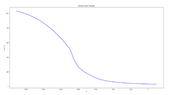
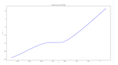
I could start with say some plots of air heat capacity and density for our range of temperatures, for a few pressures? To get an idea of how we would expect the model output to change by adding these two in. I'll add them in separately then