Numerically find the energy of the delta-well's bound state

Muizz
Messages
11
Reaction score
0
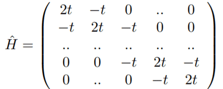
I'm working on an assignment where I'm required to numerically find the energy of a delta-potential's bound state. To do this, we've converted the time-independent schrödinger equation to an eigenvalue problem with E the eigen value, ψ the eigen vector and H a matrix as follows:
391fcef12d.png

with ##t = \frac{\hbar^2}{2ma^2}##.

Now, my specific problem is this:
3e839211e6.png


I've already done all the theoretical calculations, and am just left with figuring out the code. I've tried a bunch of things, but I haven't been able to get the bound state to appear. My code is as follows:


Python:
import numpy as np
import matplotlib
matplotlib.use("TkAgg")
import matplotlib.pyplot as plt

#################################################
# Parameter input
#################################################

hbar = 1.05e-34
h    = 6.626e-34
m    = 1
N    = 400
a    = 1
L    = N * a
t    = hbar**2 / ( 2 * m * a**2)

#################################################
# Parameter sanity check
#################################################
assert N%2 == 0, 'N must be an even number'
assert m    > 0, 'Mass must be positive'
assert a    > 0, 'Distance between points must be positive'
assert t   >= 0, 'T must be non-negative. Make sure hbar is positive.'

#################################################
# Base code
#################################################
for i in range(0,100,10):
    # Building the hamiltonian operator matrix and calculating its eigen
    # values (eval) and eigen vectors (evec)
    n  = int(N/2)
    a1 = np.full((N-1,), -t)
    a2 = np.full((N,), 2*t)
    Hamiltonian = np.diag(a1, -1) +  np.diag(a2) + np.diag(a1, 1)
    Hamiltonian[n,n] = Hamiltonian[n,n]- 1*10**i  # Adds potential in middle.
    eval, evec = np.linalg.eigh(Hamiltonian) # use .eig() if Hamiltonian is not symmetric

    plt.plot(evec)
    plt.show()
I'm quite desperate, hence the post here. Thanks in advance for all your help!

For those amongst you who'd prefer a nicely formatted image of the assignment: https://puu.sh/yKp4D/b668471918.png
 

Attachments

  • 391fcef12d.png
    391fcef12d.png
    4.9 KB · Views: 1,077
  • 3e839211e6.png
    3e839211e6.png
    52.2 KB · Views: 987
Last edited:
Physics news on Phys.org
Muizz said:
I'm working on an assignment where I'm required to numerically find the energy of a delta-potential's bound state. To do this, we've converted the time-independent schrödinger equation to an eigenvalue problem with E the eigen value, ψ the eigen vector and H a matrix as follows:
View attachment 217127
with t = [$]\frac{\hbar^2}{2ma^2}[/$].

Now, my specific problem is this:
View attachment 217128

I've already done all the theoretical calculations, and am just left with figuring out the code. I've tried a bunch of things, but I haven't been able to get the bound state to appear. My code is as follows:


Python:
import numpy as np
import matplotlib
matplotlib.use("TkAgg")
import matplotlib.pyplot as plt

#################################################
# Parameter input
#################################################

hbar = 1.05e-34
h    = 6.626e-34
m    = 1
N    = 400
a    = 1
L    = N * a
t    = hbar**2 / ( 2 * m * a**2)

#################################################
# Parameter sanity check
#################################################
assert N%2 == 0, 'N must be an even number'
assert m    > 0, 'Mass must be positive'
assert a    > 0, 'Distance between points must be positive'
assert t   >= 0, 'T must be non-negative. Make sure hbar is positive.'

#################################################
# Base code
#################################################
for i in range(0,100,10):
    # Building the hamiltonian operator matrix and calculating its eigen
    # values (eval) and eigen vectors (evec)
    n  = int(N/2)
    a1 = np.full((N-1,), -t)
    a2 = np.full((N,), 2*t)
    Hamiltonian = np.diag(a1, -1) +  np.diag(a2) + np.diag(a1, 1)
    Hamiltonian[n,n] = Hamiltonian[n,n]- 1*10**i  # Adds potential in middle.
    eval, evec = np.linalg.eigh(Hamiltonian) # use .eig() if Hamiltonian is not symmetric

    plt.plot(evec)
    plt.show()
I'm quite desperate, hence the post here. Thanks in advance for all your help!

For those amongst you who'd prefer a nicely formatted image of the assignment: https://puu.sh/yKp4D/b668471918.png

I do not see any place where you are computing an eigenvalue or an eigenvector, unless is is in a procedure that is called somewhere.

Anyway, the type of approach you attempt is quite possibly bound to fail, because of numerical scaling problems and severe roundoff error problems. Your matrix H has a possibly small entry ##t##. It is much better to set ##H = t A## where ##A## is the matrix you would get if you put ##t = 1##. Now, if ##\lambda## is an eigenvalue of ##A## and ##v## is an eigenvector, then ##t \lambda## is an eigenvalue of ##H = tA## and ##v## is an eigenvector (of both ##A## and ##H##). All the numerical work of finding eigenvalues/eigenvectors of ##A## is divorced from the numerical value of ##t##. However, you can just multiply your answer by ##t## as the very last step of you solution procedure, after all the hard work has been done.
 
According to your calculations, at what is the energy of the bound state?

By the way, it looks strange that are are using SI units for ħ but take the mass and a to be 1. I would use units such that ħ = 1.
 
Ray Vickson said:
I do not see any place where you are computing an eigenvalue or an eigenvector, unless is is in a procedure that is called somewhere.
It's the action of numpy.linalg.eigh.
 
Ray Vickson said:
I do not see any place where you are computing an eigenvalue or an eigenvector, unless is is in a procedure that is called somewhere.

Anyway, the type of approach you attempt is quite possibly bound to fail, because of numerical scaling problems and severe roundoff error problems. Your matrix H has a possibly small entry ##t##. It is much better to set ##H = t A## where ##A## is the matrix you would get if you put ##t = 1##. Now, if ##\lambda## is an eigenvalue of ##A## and ##v## is an eigenvector, then ##t \lambda## is an eigenvalue of ##H = tA## and ##v## is an eigenvector (of both ##A## and ##H##). All the numerical work of finding eigenvalues/eigenvectors of ##A## is divorced from the numerical value of ##t##. However, you can just multiply your answer by ##t## as the very last step of you solution procedure, after all the hard work has been done.
Right. That makes a lot of sense (and explains why they're telling my to vary ##V_0/t##.. Changing this little thing gets a much nicer curve, I'll still need to verify if it's the correct curve, but I call this progress :) Thanks!
Edit: Turns out I'm ~2 orders of magnitude off now.. Progress indeed.

DrClaude said:
According to your calculations, at what is the energy of the bound state?

By the way, it looks strange that are are using SI units for ħ but take the mass and a to be 1. I would use units such that ħ = 1.
That's my doing. I figured I knew ##\hbar## but not the rest so I only kept it in SI units.

According to my calculations, the bound state occurs at ##E = -\frac{m}{2\hbar^2}##. Note how I leave out a factor (as I do in my code) because I don't know how to compensate for ##\lambda\delta(x)##.
 
Last edited:
Thread 'Need help understanding this figure on energy levels'
This figure is from "Introduction to Quantum Mechanics" by Griffiths (3rd edition). It is available to download. It is from page 142. I am hoping the usual people on this site will give me a hand understanding what is going on in the figure. After the equation (4.50) it says "It is customary to introduce the principal quantum number, ##n##, which simply orders the allowed energies, starting with 1 for the ground state. (see the figure)" I still don't understand the figure :( Here is...
Thread 'Understanding how to "tack on" the time wiggle factor'
The last problem I posted on QM made it into advanced homework help, that is why I am putting it here. I am sorry for any hassle imposed on the moderators by myself. Part (a) is quite easy. We get $$\sigma_1 = 2\lambda, \mathbf{v}_1 = \begin{pmatrix} 0 \\ 0 \\ 1 \end{pmatrix} \sigma_2 = \lambda, \mathbf{v}_2 = \begin{pmatrix} 1/\sqrt{2} \\ 1/\sqrt{2} \\ 0 \end{pmatrix} \sigma_3 = -\lambda, \mathbf{v}_3 = \begin{pmatrix} 1/\sqrt{2} \\ -1/\sqrt{2} \\ 0 \end{pmatrix} $$ There are two ways...
Back
Top