How to Enhance 3D Parametric Plots in Mathematica?

In summary: The improved visual of the graphic by using some built-in commands to label curves on the surface itself. For instance, the curve on the surface be labelled \alpha (t) and is positioned along the curve somewhere.How?About the Mesh-> None problem, i used Show[c1,s1] for the individual plots. Its solves now.However, i still do not fully understand the technique of using the arrowheads. For example i usec1=ParametricPlot3D[{1+Cos[t],Sin[t],2*Sin[t/2]},{t,0,pi/2}],PlotStyle-> {Directive[Red
  • #1
Ishika_96_sparkles
57
22
TL;DR Summary
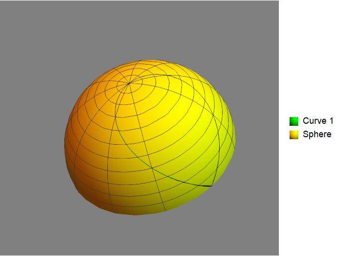
I tried to make a superimposed plot of a curve on a half sphere and need help with some graphics.
This is the code line that i used to generate the following graphs

Mathematica Code lines:
ParametricPlot3D[{{1 + Cos[t], Sin[t],
   2*Sin[t/2]}, {2 *Cos[t]*Sin[\[Phi]], 2*Sin[t]*Sin[\[Phi]],
   2*Cos[\[Phi]]}}, {t, 0, 2 \[Pi]}, {\[Phi], 0, \[Pi]/2},
 PlotStyle -> {Directive[Green, Thickness[0.025]], Yellow},
 PlotRange -> All, PlotLegends -> {"Curve 1", "Sphere"},
 BoxRatios -> {2, 2, 1}, Axes -> False, Background -> Gray,
 Boxed -> False, Mesh -> 10]

I obtained the following output

ParPlot3D.jpg


and with a slight change in the background
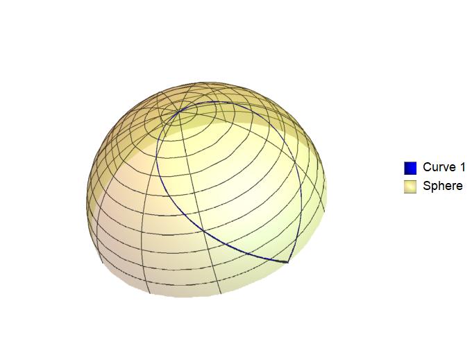
ParPlot3D2.jpg


Query:

I want to know if the visual of the general curve can be improved
and if one could put arrowheads along the Curve 1 in the anti-clockwise sense of rotation. What could be the procedure?

When I turn off the Mesh, the Curve 1 also vanishes. How could I keep the curve and put Mesh-> None at the same time?
 
Physics news on Phys.org
  • #2
Ishika_96_sparkles said:
I want to know if the visual of the general curve can be improved
How?

Ishika_96_sparkles said:
and if one could put arrowheads along the Curve 1 in the anti-clockwise sense of rotation. What could be the procedure?
See https://mathematica.stackexchange.com/questions/127415/addding-arrows-in-closed-curves

Ishika_96_sparkles said:
When I turn off the Mesh, the Curve 1 also vanishes. How could I keep the curve and put Mesh-> None at the same time?
It works when I try it.
 
  • #3
DrClaude said:

Thanks for the reply Dr Claude. I followed your link and tried to use it in my own code. I am able to get this
3Dplots.jpg
The improved visual of the graphic by using some built-in commands to label curves on the surface itself. For instance, the curve on the surface be labelled [itex]\alpha (t)[/itex] and is positioned along the curve somewhere.

About the Mesh-> None problem, i used Show[c1,s1] for the individual plots. Its solves now.

However, i still do not fully understand the technique of using the arrowheads. For example i use
Mathematica Code lines:
c1=ParametricPlot3D[{1+Cos[t],Sin[t],2*Sin[t/2]},{t,0,pi/2}],
PlotStyle-> {Directive[Red,Thickness[0.005]],Arrowheads[{0,0.05,0.05,0.05,0}]},
PlotRange-> All,BoxRatios-> {2,2,1},Boxed-> True,Axes-> True]/.Line-> Arrow

I do not understand how the replacement works in this case! i.e. /.Line-> Arrow is linked to the list of arrowheads be placed on the curve c1. How? or should I have used /.c1-> Arrow?
 
  • #4
Ishika_96_sparkles said:
Mathematica Code lines:
c1=ParametricPlot3D[{1+Cos[t],Sin[t],2*Sin[t/2]},{t,0,pi/2}],
PlotStyle-> {Directive[Red,Thickness[0.005]],Arrowheads[{0,0.05,0.05,0.05,0}]},
PlotRange-> All,BoxRatios-> {2,2,1},Boxed-> True,Axes-> True]/.Line-> Arrow
This can't be the exact code as the brackets aren't paired.

Ishika_96_sparkles said:
I do not understand how the replacement works in this case! i.e. /.Line-> Arrow is linked to the list of arrowheads be placed on the curve c1. How? or should I have used /.c1-> Arrow?
The former is the correct approach. Note however the use of :> instead of -> and the fact that it is Line[x_], not simply Line.
 
  • #5
DrClaude said:
This can't be the exact code as the brackets aren't paired.

Yes, i had typed it out by hand. Sorry for the inconvenience.

Here is all the code pasted below

Mathematica Code lines:
Clear[c1, s1]

c1 = ParametricPlot3D[{1 + Cos[t], Sin[t], 2*Sin[t/2]}, {t, 0,
     2 \[Pi]},
    PlotStyle -> {Directive[Red, Thickness[0.005]],
      Arrowheads[{0, 0.05, 0.05, 0.05, 0}]}, PlotRange -> All,
    BoxRatios -> {2, 2, 1}, Boxed -> True, Axes -> True] /.
   Line -> Arrow;

s1 = ParametricPlot3D[{2 *Cos[t]*Sin[\[Phi]], 2*Sin[t]*Sin[\[Phi]],
    2*Cos[\[Phi]]}, {t, 0, 2 \[Pi]}, {\[Phi], 0, \[Pi]/2},
   PlotStyle ->
    Directive[Yellow, Opacity[0.3], Specularity[White, 10]],
   PlotRange -> All, BoxRatios -> {2, 2, 1}, Axes -> False,
   Background -> White, Boxed -> False, Mesh -> None];

Show[{c1, s1}]

Used the Arrow part in c1.
 

1. How do I create a parametric plot in 3D?

To create a parametric plot in 3D, you will need to specify the three variables (x, y, and z) in terms of a fourth variable (usually t). Then, use a plotting software or programming language, such as MATLAB or Python, to plot the x, y, and z values for a range of t values.

2. What is the purpose of a parametric plot in 3D?

A parametric plot in 3D is used to visualize the relationship between three variables that are dependent on a fourth variable. This can be useful in understanding complex systems and patterns, as well as in mathematical modeling and data analysis.

3. How do I interpret a parametric plot in 3D?

In a parametric plot in 3D, the three axes represent the values of the variables x, y, and z. The plot will show how the values of these variables change as the fourth variable (usually t) changes. The shape and direction of the plot can provide insights into the relationship between the variables.

4. Can I customize the appearance of a parametric plot in 3D?

Yes, you can customize the appearance of a parametric plot in 3D by changing the colors, line styles, and other visual elements. This can be done in most plotting software and programming languages, by specifying the desired parameters in the plotting function or using a style sheet.

5. Are there any limitations to creating a parametric plot in 3D?

One limitation of creating a parametric plot in 3D is that it can be difficult to visualize or interpret when the relationship between the variables is complex. Additionally, the accuracy of the plot may be affected by the range of values chosen for the fourth variable and the resolution of the plot.

Similar threads

  • MATLAB, Maple, Mathematica, LaTeX
Replies
2
Views
898
  • MATLAB, Maple, Mathematica, LaTeX
Replies
1
Views
1K
  • MATLAB, Maple, Mathematica, LaTeX
Replies
4
Views
3K
  • MATLAB, Maple, Mathematica, LaTeX
Replies
1
Views
696
  • MATLAB, Maple, Mathematica, LaTeX
Replies
1
Views
2K
  • MATLAB, Maple, Mathematica, LaTeX
Replies
1
Views
2K
  • MATLAB, Maple, Mathematica, LaTeX
Replies
2
Views
1K
Replies
2
Views
1K
  • Advanced Physics Homework Help
Replies
6
Views
629
  • MATLAB, Maple, Mathematica, LaTeX
Replies
2
Views
2K
Back
Top