Series of Standing Waves in Matlab

In summary, this code creates a standing wave along a string. I need to create a few more of these, to end up with a series of standing waves which I can then calculate the sum of, which gives me the net displacement of the wave. I then need to plot this net displacement, which will result in a traveling wave.
  • #1
henrybrent
57
0
%PLOTTING TIME DEPENDENT MOTION OF A STANDING WAVE
%Define Parameters
a_n = 1;
k = 5;
w_n = 5;
x = 0:0.05:4;
t = 1:0.05:20;

for j=1:length(t)
for i=1:length(x)
u(i) = a_n*sin(k.* x(i)).* cos(w_n.*t(j)); %Formula for displacement
end
pause (0.1)
plot(u)
axis([1,65,-1.5,1.5])
grid on
end

Above is the code for a standing wave along a string. I need to create a few more of these, to end up with a series of standing waves which I can then calculate the sum of, which gives me the net displacement of the wave. I then need to plot this net displacement, which will result in a traveling wave.

Equation 1 on the formula sheet attached is the equation that governs the source that generates the series of standing waves. Tau is a 'tuning parameter'. I can just assign it a value. It determines the angular frequency. Imagine plucking a guitar. That is the source. We pluck the string of a guitar at a certain distance along the string. That distance is denoted as X_s (X subscript s). That can just be a value.

Equation 2 is the displacement for the nth standing wave (harmonic) where L is the length of the string, x is displacement and w_n (omega subscript n) is the angular frequency n is the harmonic number. I need to incorporate this somehow into the loop I have used to generate the wave in my code, in order to plot, let's say, the first 5 harmonics as subplots.

Equation 3 is then used to sum all of these harmonics together, to generate a final plot.

Any ideas on how to do this using the code and formula I have written
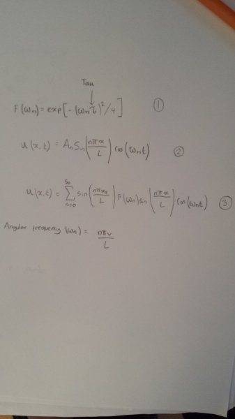
STANDINGWAVE (2).jpg
 
Physics news on Phys.org
  • #2
henrybrent said:
Above is the code for a standing wave along a string. I need to create a few more of these, to end up with a series of standing waves which I can then calculate the sum of, which gives me the net displacement of the wave. I then need to plot this net displacement, which will result in a traveling wave.

Which parameter do you think will vary to produce all of the different waves?
 
  • #3
Angular frequency/harmonic number.
 
  • #4
Yes. So you should be able to adapt your code to have a for loop that loops through different values for n, and calculates the displacement for the nth standing wave. Inside that loop is the loop over j that simulates the passage of time. I'm not sure how many values of n you'll need to use to get suitable final results (where everything is summed), so you'll have to play with that. I'd try 100 to start perhaps.

You'll also want to change the way this is visualized, since you probably do not want to visualize the standing waves one at a time.

HINT: This loop is entirely unnecessary:

for i=1:length(x)
 
  • #5
kreil said:
Yes. So you should be able to adapt your code to have a for loop that loops through different values for n, and calculates the displacement for the nth standing wave. Inside that loop is the loop over j that simulates the passage of time. I'm not sure how many values of n you'll need to use to get suitable final results (where everything is summed), so you'll have to play with that. I'd try 100 to start perhaps.

You'll also want to change the way this is visualized, since you probably do not want to visualize the standing waves one at a time.

HINT: This loop is entirely unnecessary:

for i=1:length(x)
using the i=1:length(x) was only way I could figure out how to animate the wave.

I'm aware of what I need to do regarding n, but I wasn't too sure how to implement it. I'm not very strong with Matlab, but unfortunately it is all I have at the moment. later for my research work I'll be working in a unix environment, but for now it's matlab!
 
  • #6
Here is a good starting point to continue from. This code runs but still needs a lot of work. Let me know if you have any questions!

Code:
%PLOTTING TIME DEPENDENT MOTION OF A STANDING WAVE
%Define Parameters
a_n = 1;
k = 5;
L = 1;
w_n = @(n,x,t) n*pi.*x./L.*t;
x = 0:0.01:4;
t = 1:0.001:20;

for j=1:length(t)
    u = a_n*sin(k.* x).* cos(w_n(j,x,t(j)).*t(j)); %Formula for displacement
    pause (0.1)
    plot(u)
    axis([1,65,-1.5,1.5])
    grid on
end
 
Last edited:
  • #7
kreil said:
Here is a good starting point to continue from. This code runs but still needs a lot of work. Let me know if you have any questions!

Code:
%PLOTTING TIME DEPENDENT MOTION OF A STANDING WAVE
%Define Parameters
a_n = 1;
k = 5;
L = 1;
w_n = @(n,x,t) n*pi.*x./L.*t;
x = 0:0.01:4;
t = 1:0.001:20;

for j=1:length(t)
    u = a_n*sin(k.* x).* cos(w_n(j,x,t(j)).*t(j)); %Formula for displacement
    pause (0.1)
    plot(u)
    axis([1,65,-1.5,1.5])
    grid on
end

So this is where I apply the loop over the initial loop for n = 1:4, to separate the harmonics. The code looks like a load of harmonics looping over and over again.
 
  • #8
Would Indexing instead of using nested for loops be a better/more efficient way of doing this?
 
  • #9
henrybrent said:
Would Indexing instead of using nested for loops be a better/more efficient way of doing this?

I'd advise against optimizing a program that isn't fully written. For your application, it's more important that the program runs and produces correct results.

While it's true that vectorized code will generally run faster in MATLAB than equivalent code that uses loops, for small applications like this the difference will be pretty insignificant. So ultimately your choice to use one or the other at this point should be entirely based on what you're more comfortable working with.
 
  • #10
Ok, that makes sense.

What is K in your formula?

In mine, it was to represent n*pi/L, just a constant in my mind, but obviously that's wrong. In your code its still present as k=5?
 
  • #11
I just left k alone, but you can and should update it to be equal to n*pi/L, where "n" is an input variable that can change. Then you can update the definition of w_n to use k.
 
  • #12
k = n*pi/L
w_n = @(n,x,t) (k*x)*t;

Getting a dimensional error
 
  • #13
henrybrent said:
k = n*pi/L
w_n = @(n,x,t) (k*x)*t;

Getting a dimensional error

You'll want to use function handles, so that when you call k(n) it evaluates k for that value of n. In these expressions the @(...) expression defines what the variables (inputs) are.

Code:
k = @(n) n*pi/L;
w_n = @(n,x,t) k(n).*x./t;

Now, since k and w_n are function handles, you always need to call them with the proper inputs. So anywhere there is a k should be replaced by k(n), and anywhere there is w_n should be replaced by w_n(n,x,t).

Also, notice that n is not a variable in your workspace based on these lines of code. It was used passively to define a variable in the function handles, but that's it. Really these could have used anything, like z or P, but the n is suggestive. Later on when you have a loop over values of n, you can call k(n) without conflict.
 
  • #14
kreil said:
You'll want to use function handles, so that when you call k(n) it evaluates k for that value of n. In these expressions the @(...) expression defines what the variables (inputs) are.

Code:
k = @(n) n*pi/L;
w_n = @(n,x,t) k(n).*x./t;

Now, since k and w_n are function handles, you always need to call them with the proper inputs. So anywhere there is a k should be replaced by k(n), and anywhere there is w_n should be replaced by w_n(n,x,t).

Also, notice that n is not a variable in your workspace based on these lines of code. It was used passively to define a variable in the function handles, but that's it. Really these could have used anything, like z or P, but the n is suggestive. Later on when you have a loop over values of n, you can call k(n) without conflict.

Code:
a_n = 1;

L = 1;
k(n) = @(n) n*pi/L;
w_n = @(n,x,t) k(n).*x./t;

x = 0:0.05:4;
t = 1:0.01:20;

for n = 1:4
 
   for j=1:length(t)
    u = a_n*sin(k(n)* x).* cos(w_n(j,x,t(j)).*t(j)); %Formula for displacement
    pause (0.1)
    plot(u)
    axis([1,65,-1.5,1.5])
    grid on
    end

end

Atm, this is what I have down; trying to loop over the first four values of n.

This just subtitutes 1 - 4 into each iteration (I hope) and represents the harmonic number.

But I still don't get how I'd use the subplot command to somehow split each harmonic up? Meshgrid?
 
Last edited:
  • #15
I did some MATLAB visualizations in a PF insights post I wrote, and the code for the subplot animations is here:

https://physicsforums-bernhardtmedi...ontent/uploads/2015/05/CODEparticle2D_ALL.txt

In this case, the standing waves are really time independent (the denominator of w_n cancels the time in the expression for u), so you don't even need an animation. For example:

Code:
a_n = 1;

L = 1;
k = @(n) n*pi/L;
w_n = @(n,x,t) k(n).*x./t;

x = 0:0.05:4;
t = 1:0.01:20;

u = @(n,x,t) a_n*sin(k(n)* x).* cos(w_n(n,x,t).*t);

figure
subplot(2,2,1)
plot(u(1,x,t(1)))
subplot(2,2,2)
plot(u(2,x,t(1)))
subplot(2,2,3)
plot(u(3,x,t(1)))
subplot(2,2,4)
plot(u(4,x,t(1)))
 
  • #16
kreil said:
I did some MATLAB visualizations in a PF insights post I wrote, and the code for the subplot animations is here:

https://physicsforums-bernhardtmedi...ontent/uploads/2015/05/CODEparticle2D_ALL.txt

In this case, the standing waves are really time independent (the denominator of w_n cancels the time in the expression for u), so you don't even need an animation. For example:

Code:
a_n = 1;

L = 1;
k = @(n) n*pi/L;
w_n = @(n,x,t) k(n).*x./t;

x = 0:0.05:4;
t = 1:0.01:20;

u = @(n,x,t) a_n*sin(k(n)* x).* cos(w_n(n,x,t).*t);

figure
subplot(2,2,1)
plot(u(1,x,t(1)))
subplot(2,2,2)
plot(u(2,x,t(1)))
subplot(2,2,3)
plot(u(3,x,t(1)))
subplot(2,2,4)
plot(u(4,x,t(1)))

I ran your code, it looks/runs great.

My standing waves should be depending on at least the tuning parameter used in equation 1 on the sheet I attached. The standing waves result due to a source being applied (equation 1). The angular frequency is a variable that changes, yes, but I think this change is because of the relationship between the tuning parameter (tau) and angular frequency (w_n). I don't think I can/should define w_n = @(n,x,t) k(n).*x./t;

I'm still quite unsure how to approach this problem,

I have a source applied to a string, for example, that is given by equation 1. This generates a series of standing waves. I want to then subplot the first 5 harmonics of the standing waves.

Then sum them upto...100? And plot this result, this should end up with a traveling wave. (I think).

At the moment, I have a standing wave generating 4 harmonics. But not a standing wave as a result of a source applied.
 
  • #17
henrybrent said:
My standing waves should be depending on at least the tuning parameter used in equation 1 on the sheet I attached. The standing waves result due to a source being applied (equation 1). The angular frequency is a variable that changes, yes, but I think this change is because of the relationship between the tuning parameter (tau) and angular frequency (w_n). I don't think I can/should define w_n = @(n,x,t) k(n).*x./t;

Your equation for w_n did not depend on tau, so what is their relationship to each other? You're correct that my definition of w_n is probably not right, as the velocity v depends on the wavelength and frequency (I did this quickly and just used x and t).

henrybrent said:
I'm still quite unsure how to approach this problem,

I have a source applied to a string, for example, that is given by equation 1. This generates a series of standing waves. I want to then subplot the first 5 harmonics of the standing waves.

Equation 1 describes an exponentially decreasing force, yes? Since w_n is inversely proportional to time, then as t goes to infinity w_n goes to zero and F settles on a value of 1. I haven't studied standing waves extensively, so I assumed the second equation resulted from the first and was the one we wanted to use. Otherwise, what do you hope to do with these values of F?

henrybrent said:
Then sum them upto...100? And plot this result, this should end up with a traveling wave. (I think).

At the moment, I have a standing wave generating 4 harmonics. But not a standing wave as a result of a source applied.

I believe your problems right now are with the physics and not with the code. Except for the source, the rest of the problem is mostly solved, and the last part of summing the harmonics and plotting the time simulation should be straightforward as well.
 
  • #18
The equation used to describe the standing wave is
kreil said:
Your equation for w_n did not depend on tau, so what is their relationship to each other? You're correct that my definition of w_n is probably not right, as the velocity v depends on the wavelength and frequency (I did this quickly and just used x and t).
Equation 1 describes an exponentially decreasing force, yes? Since w_n is inversely proportional to time, then as t goes to infinity w_n goes to zero and F settles on a value of 1. I haven't studied standing waves extensively, so I assumed the second equation resulted from the first and was the one we wanted to use. Otherwise, what do you hope to do with these values of F?
I believe your problems right now are with the physics and not with the code. Except for the source, the rest of the problem is mostly solved, and the last part of summing the harmonics and plotting the time simulation should be straightforward as well.

The code for the standing wave uses equation

[itex] u(x,t) = A_nsin(\frac{n \pi x}{L})cos(\omega_n t)[/itex]

where [itex] \omega_n = \frac{n\pi v x}{L} [/itex]

the source is described as [itex]F( \omega_n) = e^\frac{ {(- \omega_n \tau)^2}}{4} [/itex]
When the source is applied at distance [itex]x_s[/itex], then the net displacement (sum of the standing waves) is given by the expression

[itex]u(x,t) = \sum\limits_{n=0}^{\infty} \sin(\frac{n\pi x_s}{L})F(\omega_n)\sin(\frac{n\pi x}{L})\cos(\omega_nt)[/itex]
 
  • #19
Alright, thanks for the clarification. Let's just get the goals solidified quickly to make sure we're on track (correct me where I'm wrong):

1. Use the equation for the standing wave harmonics and plot time simulations of the first 5 harmonics in subplots:
[tex]
u(x,t) = A_n \sin \left( \frac{n \pi x}{L} \right) \cos(\omega_n t)
[/tex]

2. Then, use the net displacement equation to plot the net displacement below the harmonic subplots.
[tex]
u(x,t) = \sum\limits_{n=0}^{\infty} \sin \left( \frac{n\pi x_s}{L} \right) F(\omega_n)\sin(\frac{n\pi x}{L})\cos(\omega_nt)
[/tex]

Is that all? If so, we've essentially finished the first task and just need to do the second. It doesn't appear that the second step uses any of the results from the first step, though. Is there an expression for A_n that is missing here?
 
  • #20
kreil said:
Alright, thanks for the clarification. Let's just get the goals solidified quickly to make sure we're on track (correct me where I'm wrong):

1. Use the equation for the standing wave harmonics and plot time simulations of the first 5 harmonics in subplots:
[tex]
u(x,t) = A_n \sin \left( \frac{n \pi x}{L} \right) \cos(\omega_n t)
[/tex]

2. Then, use the net displacement equation to plot the net displacement below the harmonic subplots.
[tex]
u(x,t) = \sum\limits_{n=0}^{\infty} \sin \left( \frac{n\pi x_s}{L} \right) F(\omega_n)\sin(\frac{n\pi x}{L})\cos(\omega_nt)
[/tex]

Is that all? If so, we've essentially finished the first task and just need to do the second. It doesn't appear that the second step uses any of the results from the first step, though. Is there an expression for A_n that is missing here?

Almost, rather than think of it as two problems, I'm thinking of it as just 1.
Write a script that sums the first 100? harmonics of the string when the source is applied, and plot the first 5 harmonics as well as the combination of 100.

I should be able to use just the equation for the source [itex]F(\omega_n)[/itex] and the expression for net displacement to solve this problem.

EDIT: just to confirm, this is time dependent motion of waves I'm looking at.
 
Last edited:
  • #21
I should be able to use just the equation for the source F(ωn) and the expression for net displacement to solve this problem.

I believe you use that equation for the net displacement (sum of 100 or so harmonics), but for the individual harmonics (plotting the first 5 harmonics) you need to use the other equation for u(x,t), right? This is why I said the results aren't really related to each other before.

I have some code I've been working on but can't post it until later today. In the meantime, post any new code you've been working on for this problem.
 
  • #22
[itex]
u(x,t) = \sum\limits_{n=0}^{\infty} \sin \left( \frac{n\pi x_s}{L} \right) F(\omega_n)\sin(\frac{n\pi x}{L})\cos(\omega_nt)
[/itex]

I think this is the equation we use.

However, to plot the first few harmonics, we just use [itex]\sin \left( \frac{n\pi x_s}{L} \right) F(\omega_n)\sin(\frac{n\pi x}{L})\cos(\omega_nt)[/itex] and set n = 1, 2, 3, 4, 5 etc and plot those .

THEN we can use the summation, and then plot that? I think that's easier (and correct, as this is the equation that involves the source, which is vital)
 
  • #23
Ok, I'll incorporate that into the code I'm working on.
 
  • #24
Ok, thank you
 
  • #25
Still haven't managed to solve this. Will post what I've got soon when I'm home
 
  • #26
I don't have time to finish this so I'll just post what I have so far and let you work on it.

Code:
% Constants and variables
a_n = 1;
L = 1;
x_s = 0.5;
tau = 4;
v = 1;
k = @(n) n*pi/L;
w_n = @(n,v) k(n).*v;

% Time and position durations
x = linspace(0,4,1000);
t = linspace(0,20,1000);

% Define the source
F = @(w) exp(-(w.*tau/2).^2);

% Define the displacement
u = @(n,v,t) sin(k(n).*x_s).*F(w_n(n,v)).*sin(k(n).*x).*cos(w_n(n,v).*t);
figure

% Simulate the first four harmonics
for j = 1:length(t)
    subplot(2,2,1)
    q = u(1,1,t(j));
    plot(x,q)
    ylim([-1e-17 1e-17])
    title('n=1')
   
    subplot(2,2,2)
    q = u(2,1,t(j));
    plot(x,q)
    ylim([-0.5e-84 0.5e-84])
    title('n=2')
   
    subplot(2,2,3)
    q = u(3,1,t(j));
    plot(x,q)
    ylim([-6e-155 6e-155])
    title('n=3')
   
    subplot(2,2,4)
    q = u(4,1,t(j));
    plot(x,q)
    ylim([-1.5e-290 1.5e-290])
    title('n=4')
   
    drawnow
end

This simulates the first four harmonics. To get the net displacement over time, my strategy was use two for loops: the first over time, the second over n. For each time step, you loop through all n values and add each answer to the previous one. At the end of each loop over n, you have summed up the net displacement for that time step and can plot it. So the result is that you get to watch the net displacement change over time.
 
  • #27
so how can we write this code for standing water waves?
 
  • #28
Still haven't cracked it, haven't had time to work on it.
 

What is a series of standing waves in Matlab?

A series of standing waves in Matlab is a simulation of a physical phenomenon where multiple waves with the same frequency and amplitude interfere with each other, resulting in stationary points of maximum and minimum amplitude. This can be visualized as a pattern of peaks and troughs that do not move over time.

How does Matlab represent a series of standing waves?

Matlab represents a series of standing waves as a combination of sine and cosine functions, where the amplitude and phase of each function determines the shape of the standing wave. The sum of these functions creates the overall pattern of the standing waves.

What can a series of standing waves in Matlab be used for?

A series of standing waves in Matlab can be used for a variety of purposes, such as studying wave interference and resonance, analyzing vibrations in mechanical systems, and designing antennas and other wave-based technologies.

How can I create a series of standing waves in Matlab?

To create a series of standing waves in Matlab, you can use the "plot" function to plot the individual sine and cosine functions, and then use the "hold on" command to combine them into one graph. You can also adjust the parameters of the functions to customize the shape and behavior of the standing waves.

What are some common challenges when working with series of standing waves in Matlab?

Some common challenges when working with series of standing waves in Matlab include understanding the underlying mathematical concepts, determining the appropriate parameters to create a desired pattern, and troubleshooting errors or unexpected behavior in the simulation. It can also be challenging to interpret and analyze the data from a series of standing waves, as it may involve complex calculations and visualizations.

Similar threads

  • Introductory Physics Homework Help
Replies
19
Views
320
  • MATLAB, Maple, Mathematica, LaTeX
Replies
1
Views
1K
  • MATLAB, Maple, Mathematica, LaTeX
Replies
8
Views
1K
Replies
41
Views
14K
Replies
19
Views
1K
  • MATLAB, Maple, Mathematica, LaTeX
Replies
2
Views
2K
  • MATLAB, Maple, Mathematica, LaTeX
Replies
1
Views
745
  • MATLAB, Maple, Mathematica, LaTeX
Replies
2
Views
2K
  • MATLAB, Maple, Mathematica, LaTeX
Replies
10
Views
2K
  • MATLAB, Maple, Mathematica, LaTeX
Replies
6
Views
2K
Back
Top